Introduction to subspace methods
Background
In the discussion of early color vision, we explored the way that multi-dimensional optical spectra are projected by the human visual system into a three-dimension subspace. Human retinal cones have three light-sensitive pigments, each with a different spectral sensitivity, and thus the encoding of colors in the retina by the responses of these three pigments can only span a three-dimensional space. Despite the fact that the cell responses are highly non-linear, the overall system behaves in a remarkably linear way, at least when examined in classical color-matching experiments.
We can focus on two different aspects of this situation. One is dimensionality reduction: human perception of colors "lives" in a space with only three dimensions, even though electromagnetic radiation (in the visible-light region of the spectrum) has many more degrees of freedom than that, so that lights with very different spectra can be "metamers". Another is change of coordinates: the natural dimensions of early color vision are not the frequencies of visible light, but the spectral sensitivities of the retinal pigments.
In dealing with any sorts of multi-dimensional data, it is often helpful to find a new coordinate system, different from the one in which the data initially presents itself. This new coordinate system might be chosen because its basis vectors have particularly useful mathematical properties, independent of the specific properties of the data set being analyzed. As we saw earlier, this is the case for Fourier coefficients: because sinusoids are eigenfunctions of linear shift-invariant systems, a set of coordinates with sinusoids as basis vectors reduces the effect of an LSI to element-wise multiplication rather than overall convolution. "Wavelets" have similar properties, adding the benefit of locality in time (and/or space) as well as frequency.
Alternatively, we might choose our new coordinate system in a data-dependent way, so as to optimally match some structure found in the data itself. We might do this because the result allows us (or more likely, a computer algorithm) to "see" patterns in the data more clearly; we might also do it because in the new coordinate system, we can represent the data more succinctly, throwing away many or even most of the apparent degrees of freedom in the original representation.
This lecture presents a general framework for thinking about data-dependent choices of coordinate systems.
One warning: although these techniques are widely applicable and can be very effective, they are also very limited. Given a body of observations described as vectors, they can provide a new descriptions in terms of vectors whose elements are linear combinations of the elements of the original vectors. (There are also a few pre-processing steps that can sometimes help to make such techniques work better, such as subtracting averages to center the data on the origin, or "sphering" the data to remove correlations).
There are many ways to do this, and often the techniques are spectacularly effective. It's easy, all the same, to create or find data sets whose instrinsic structure is not revealed by choosing a new set of basis vectors, and indeed in some cases the results of the kind of analysis we are considering here might be to introduce unpleasant artifacts that obscure what is really going on. We'll close the lecture with an example of this type.
Many interesting interesting and important techniques center around the ideas of embedding of a set of points in a higher-dimensional space, or projecting a set of points into a lower-dimensional space.
It's important to become comfortable with these geometical ideas and with their algebraic (and computational) counterparts.
Projecting a point onto a line
Suppose that we have a point b in n-dimension space -- that is, a (column) vector with n components -- and we want to find its distance to a given line, say the line from the origin through the point a (another column vector with n components). We want the point p on the line through a that is closest to b. (The point p is also the projection of the point b onto the line through a.)
It should be obvious to your geometrical intuition that the line from point b to point p is perpendicular to the line defined by a.
It should be obvious to your algebraic intution that any point on the line through point a can be represented as c*a, for some scalar c. Another simple fact of the algebra of vectors is that the line from point b to point c*a is b-c*a.
Since the vector b-c*a must be perpendicular to the vector a, it follows that their inner product must be 0. Thus (in Matlab-ese)
a'*(b-c*a) = 0
and therefore, with a bit of algebraic manipulation,
a'*b - c*a'*a = 0
a'*b = c*a'*a
c = (a'*b)/(a'*a)
This allows us to compute the location of p and the distance from b to a.
If we write the formula in the order
p = a*c
and substitute as above to get
p = a*(a'*b)/(a'*a)
we can re-arrange the terms (since a'*a is just a scalar) to yield
p = ((a*a')/(a'*a))*b
This is the vector b pre-multiplied by the term (a*a')/(a'*a). What is the dimensionality of that term? Well, given that a is an n-by-1 column vector, we have
(n-by-1 * 1-by-n)/(1-by-n * n-by-1)
or
(n-by-n)/(1-by-1)
or just n-by-n.
In other words, we're projecting point b onto the line through point a by pre-multiplying b by an n-by-n projection matrix (call it P), which is particularly easy to define:
P = (a*a')/(a'*a)
You can forget the derivation, if you want (though it's good to be able to do manipulations of this kind), and just remember this simple and easy formula for a projection matrix.
Note that this works for vectors in a space of any dimensionality.
Note also that if we have a collection of m points B, arranged in the columns of an n-by-m matrix, then we can project them all at once by the simple matrix multiplication
B1 = P*B
which produces a new n-by-m matrix B1 whose columns contain the projections of the columns of B.
Embedding: losing a line and finding it again
Let's start with a simple and coherent set of numbers: the integers from 1 to 100:
X = 1:100;
If we add a couple of other dimensions whose values are all zero:
Xhat = [X; zeros(1,100); zeros(1,100)]';
the nature of the set remains clear by simple inspection of the matrix of values:
>> Xhat(1:10,:)

ans =

     1     0     0

     2     0     0

     3     0     0

     4     0     0

     5     0     0

     6     0     0

     7     0     0

     8     0     0

     9     0     0

    10     0     0
But now let's apply a random linear transformation (implemented as multiplication by a random 3x3 matrix)
R = rand(3);
RXhat = (R*Xhat')';
[Note that before multiplying by R, we transpose Xhat so that the rows are the feature dimensions and the columns are the observations, to make it possible to manage the linear transformation in the canonical way. Here that means to multiply a 3x3 matrix (R) by a 3x100 matrix (Xhat') to yield another 3x100 matrix, whose columns are the columns of Xhat' transformed by R. Then we transpose back, in order to get the our data back into the tradition observations-in-rows form.]
Now it's not quite so clear what we started with, just from inspection of the numbers:
>> RXhat(1:10,:)
ans =
    0.3043    0.2909    0.2425
    0.6086    0.5817    0.4850
    0.9129    0.8726    0.7275
    1.2172    1.1634    0.9701
    1.5215    1.4543    1.2126
    1.8258    1.7452    1.4551
    2.1301    2.0360    1.6976
    2.4344    2.3269    1.9401
    2.7387    2.6177    2.1826
    3.0430    2.9086    2.4252
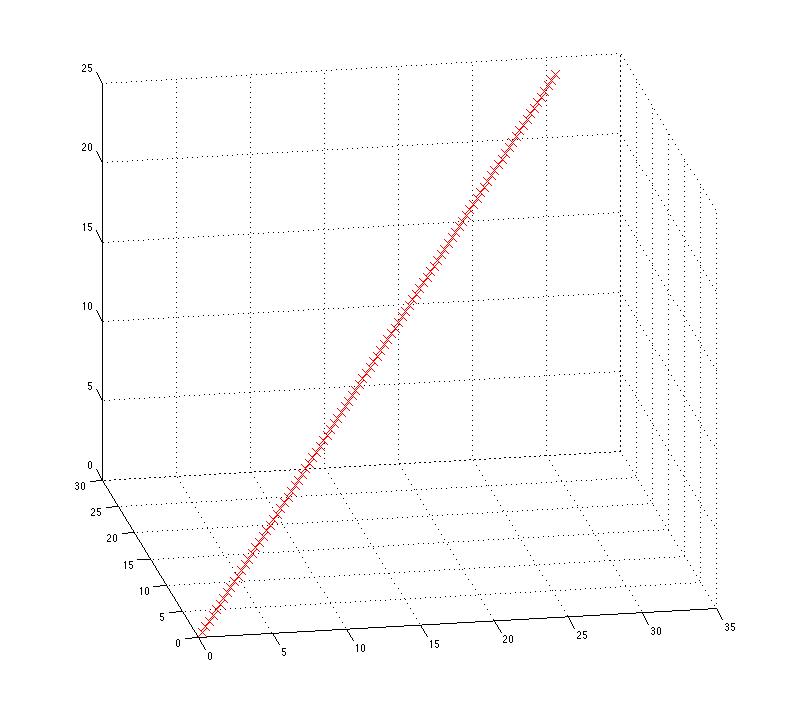
We've embedded the one-dimensional set of points in a three-dimensional space, and after the random linear transformation, the description of the points seems to use all three dimensions. But the structure -- the fact that all the data points fall on a single line -- is still evident in a 3-D plot:
plot3(RXhat(:,1),RXhat(:,2),RXhat(:,3),'rx')
grid on
Note that this structure is not dependent on the order of the (now three-dimensional) observations. We can scramble the order of the rows in RXhat without changing the plot at all -- since are just plotting the relationship among the columns, which is unchanged by the permutation:
PRXhat = RXhat(randperm(100),:);
How can we "see" mathematically what we can see visually?
One approach is to look at the singular value decomposition of the data matrix.
% First remove the column means:
MPRXhat = PRXhat-repmat(mean(PRXhat),100,1);
[U,S,V] = svd(MPRXhat');
(We remove the column means before doing the svd, because the svd deals only with rotations of the coordinate system, and an additive shift of the data -- a translation -- might in general throw it off, though it wouldn't do so in this case.)
If we look at (the first few columns of) the S matrix, we can see the evidence that this matrix of apparently 3-dimensional points is really only 1-dimensional:
>> S(:,1:5)
ans =
  140.2343         0         0         0         0
         0    0.0000         0         0         0
         0         0    0.0000         0         0
The columns of the U matrix contain the singular vectors, the basis vectors of the rotated version of the data in which the second and third dimensions shrink to zero:
>> U
U =
   -0.6264    0.2230   -0.7470
   -0.5987   -0.7512    0.2778
   -0.4992    0.6212    0.6041
So we should be able to see that the svd has found our line by creating a projection matrix from the first column of U:
U1 = U(:,1);
P = (U1*U1')/(U1'*U1);
and then projecting a suitable point onto that line, and plotting it with our embedded data:
p = P*[25 25 25]';
hold on
plot3([0 p(1)], [0 p(2)], [0 p(3)], 'bo-','LineWidth', 2)

Principal Components Analysis (PCA)
What we've just done is equivalent to (finding the first principal component) in Principal Components Analysis, often abbreviated as PCA.
PCA is a linear transformation that rigidly rotates the coordinates of a given set of data, so as to maximize the variance of the data in each of the new dimensions in succession.
Thus the first new axis is chosen so that the variance of the data (when projected along that line) is greater than for any other possible axis. The second axis is chosen from among the lines orthogonal to the first axis, so as to soak up as much as possible of the remaining variance. And so on, though the n dimensions.
(In fact the transformation is typically all calculated at once; but the effect is the same, since the singular vectors -- the new basis vectors in the columns of U -- are sorted in order of the size of their singular values -- the scalars on the diagonal of S, that express how much of the variance is taken up by each new dimension.)
As a result, it's often possible to describe the data in a lower-dimensional space, retaining only the first few of the principal components, and discarding the rest.
Let's go through the same exercise as before, but this time we'll add some noise to make it more interesting.
XXhat = [1:100; zeros(1,100); zeros(1,100)]' + 10*randn(100,3);
RXXhat = (R*XXhat')';
PRXXhat = RXXhat(randperm(100),:);
plot3(PRXXhat(:,1),PRXXhat(:,2),PRXXhat(:,3),'rx','Markersize',12);
grid on

The same technique will work to find the (first) principal component:
% First remove the column means:
MPRXXhat = PRXXhat-repmat(mean(PRXXhat),100,1);
[U,S,V] = svd(MPRXXhat');
U1 = U(:,1);
P = (U1*U1')/(U1'*U1);
p = P*[25 25 25]';
hold on
plot3([0 p(1)], [0 p(2)], [0 p(3)], 'bo-','LineWidth', 2)

If we had built some additional (linear) structure into our original fake data, it would appear in the remaining principal components (i.e. the rest of the columns of U).
Using the covariance matrix
There's an additional important trick available here.
The fake data set that we just analyzed involved 100 "observations" of 3 "features" or "variables". Exactly the same procedure would have worked if we had 270 observations of 9 features, or 1,650 observations of 23 features, or whatever.
However, as the number of rows in our data matrix increases, the svd becomes increasingly cumbersome. For a data matrix X of n (observation) rows by m (variable) columns, we transpose X and get [U,S,V] = svd(X') as
orthogonal |
diagonal |
orthogonal |
As the number of observations increases -- and n might have tens of thousands or millions of items in it, for some applications -- S and V will become unpleasantly large.
This is too bad, because for this application, we don't care about most of S or about any of V.
Luckily, there's an easy solution.
If we first calculate the covariance matrix of X, then the U matrix for the SVD of the covariance of X is the same as the U matrix for X itself.
I'm not going to try to prove this algebraically -- you can look it up in a good linear algebra textbook -- but I'll demonstrate it to you by example:
>> X = rand(100,3);
>> MX = X-repmat(mean(X),100,1);
>> CX = cov(X);
>> [U, S, V] = svd(MX');
>> [CU, CS, CV] = svd(cov(X));
>> U
U =
   -0.5714    0.2271   -0.7886
    0.7768   -0.1605   -0.6090
   -0.2649   -0.9606   -0.0847
>> CU
CU =
   -0.5714    0.2271   -0.7886
    0.7768   -0.1605   -0.6090
   -0.2649   -0.9606   -0.0847
Since the covariance matrix is a square matrix whose dimensions depend only on the number of "features" or "variables", not on the number of "observations", and since the covariance matrix remains relatively easy to compute as the number of "observations" increases, this is a good way to calculate the PCA.
(Principal Components Analysis is also sometimes referred to as the (discrete) Karhunen-Loève transform, the Hotelling transform or proper orthogonal decomposition.)
(This might be a good time to review the material on eigenvalues and eigenvectors in the Linear Algebra Review lecture notes.)
Matlab's princomp()
Note that Matlab provides a function for doing PCA:
 PRINCOMP Principal Components Analysis.
    COEFF = PRINCOMP(X) performs principal components analysis on the N-by-P
    data matrix X, and returns the principal component coefficients, also
    known as loadings.  Rows of X correspond to observations, columns to
    variables.  COEFF is a P-by-P matrix, each column containing coefficients
    for one principal component.  The columns are in order of decreasing
    component variance.

    PRINCOMP centers X by subtracting off column means, but does not
    rescale the columns of X.  To perform PCA with standardized variables,
    i.e., based on correlations, use PRINCOMP(ZSCORE(X)).  To perform PCA
    directly on a covariance or correlation matrix, use PCACOV.

    [COEFF, SCORE] = PRINCOMP(X) returns the principal component scores,
    i.e., the representation of X in the principal component space.  Rows
    of SCORE correspond to observations, columns to components.

    [COEFF, SCORE, LATENT] = PRINCOMP(X) returns the principal component
    variances, i.e., the eigenvalues of the covariance matrix of X, in
    LATENT.
The "coefficients" matrix returned by princomp() has the new basis vectors in its columns:
>> X = rand(100,3);
>> CX = cov(X);
>> [U,S,V] = svd(CX);
>> [coeff, score] = princomp(X);
>> U
U =
   -0.6973    0.2831    0.6585
   -0.6403    0.1668   -0.7498
   -0.3221   -0.9445    0.0649
>> coeff
coeff =
    0.6973   -0.2831    0.6585
    0.6403   -0.1668   -0.7498
    0.3221    0.9445    0.0649
(Note that algorithmic differences can flip the basis vectors through 180 degrees, i.e. change the sign of all the components -- two vectors pointing in opposite directions define the same line.)
The "scores" matrix has the data points as represented in the rotated space:
>> score(1:5,:)
ans =
   -0.4053    0.0377   -0.2467
   -0.3714    0.3290   -0.0826
   -0.1221    0.0971   -0.0461
    0.3198   -0.0446    0.1188
   -0.1265   -0.1299   -0.1195
>> MX = X-repmat(mean(X),100,1);  % remove column means
>> PX = (coeff'*MX')';
>> PX(1:5,:)
ans =
   -0.4053    0.0377   -0.2467
   -0.3714    0.3290   -0.0826
   -0.1221    0.0971   -0.0461
    0.3198   -0.0446    0.1188
   -0.1265   -0.1299   -0.1195
The "Fourier Expansion" equation
Let's think in a more general way about the problem of finding new dimensions in a data set.
We start with a set of observations expressed as vectors. In the cases we're thinking about now, the observations are fairly high-dimensional (i.e. each observation vector has a lot of elements).
The numbers in these observation vectors could represent anything at all: pictures of faces, EEG recordings, acoustic spectra of vowels, signals from different microphones, etc.. The general idea is to find a "natural" set of coordinates for this body of data, and to use this to produce a reduced-dimensional representation by linear projection into a subspace.
Location in the subspace is then used as a basis for measuring similarity among observations, assigning them to categories, or whatever. The motivation for the dimension reduction may be efficiency (less memory, faster calculations), or better statistical estimation (e.g. of distributions by observation type), or both.
A new set of coordinates (for an N-dimensional vector space) is equivalent to a set of N orthonormal basis vectors b1 ... bn. We can transform a vector x to the new coordinate system by multiplying x by a matrix B whose rows are the basis vectors: c = Bx. We can think of the elements of c as the values of x on the new dimensions -- or we can think of them as "coefficients" telling us how to get x back as a linear combination of the basis vectors b1 ... bn.
In matrix terms, x = B'c, since the basis vectors will be columns in B', and the expression B'c will give us a linear combination of the columns of B' using c as the weights. (Note that for typographical convenience, we're using ' to mean "transpose" in the body of the text here).
So far this is completely trivial -- we've shown that we can represent x as x = B'Bx, where B is an orthogonal matrix (and hence its inverse is its transpose).
We can re-express this in non-matrix terms as
 (Equation
1)
(Equation
1)
This is equation is known as the Fourier expansion. In actual Fourier analysis (as we'll learn soon), the basis vectors bi are sinusoids, established independent of the data being modeled -- but nothing about equation 1 requires this choice. In this lecture, we're interested in cases where we choose the basis vectors in a way that depends on the data we're trying to model -- and therefore (we hope) tells us something interesting about the structure of the phenomenon behind the measurements.
For a given orthonormal basis, the coefficients are unique -- there is a unique way to represent an arbitrary x as a linear combination of the new basis vectors B. The representation is also exact -- ignoring round-off errors, transforming to the new coordinates and then transforming back gets us exactly the original data.
Let's spend a minute on the relationship of equation 1 to the matrix form x = B'Bx. The subexpression Bx, which is giving us the vector of "coefficients" (i.e. the new coordinates), is equivalent to the subexpression read "x transpose times b sub i", which is giving us a single coefficient for each value of the index i. Spend a couple of minutes to make sure that you understand why these two equations mean the same thing.
If we truncate Equation 1 after p terms (p < N), we get
 (Equation
2)
(Equation
2)
We are thus approximating x as a linear combination of some subset of orthogonal basis vectors -- we are projecting it into a p-dimensional subspace. Obviously each choice of p orthonormal vectors gives a different approximation.
Within this general range of approaches, there are a lot of alternative criteria that have been used for choosing the set of basis vectors. Oja (Subspace Methods of Pattern Recognition, 1983) gives six:
- minimum approximation error (least average distance between x and x hat)
- least representation entropy
- maximally uncorrelated coefficients (with each other)
- maximum variances of the coefficients
- maximum separation of two classes in terms of distance in a single subspace
- maximum separation of two classes in terms of approximation errors in two subspaces
There are plenty of other criteria that have been proposed and used as well, for example maximum statistical independence of the coefficients, which gives rise to Independent Components Analysis (ICA). And Canonical Correlation Analysis, originally proposed by Hotelling in 1936, has recently been revised at Penn, e.g. in Lyle Ungar, "A vector space model of semantics using Canonical Correlation Analysis", 2013.
Often, researchers will define a criterion for choosing basis vectors that incorporates a loss function (i.e. a metric on errors) that is specific to their application. These criteria (and the associated optimization techniques for applying them to find the best-scoring subspace) can become very complex. However, in the end, it all comes down to a simple application of x=B'Bx.
Eigenfaces
This is a simple (but surprisingly effective) application of PCA by Turk and Pentland ("Eigenfaces for Recognition," J. Neuroscience, 3(1), 1991).
We start with m q x q pixel images, each arranged as an n=(q^2)-element vector by stringing the pixel values out in row ordering, starting from the upper left of the image. This is the standard way of treating images as vectors. Call these image vectors G1 ... Gm. Note that n will be fairly large: e.g. if q = 256, n = 65,536.
Calculate the "average face" F -- just the element-wise average pixel value -- and subtract it out from all the images, producing a set of mean-corrected image vectors H1 ... Hm = G1-F ... Gm-F.
Calculate the covariance matrix C of the mean-corrected images. If L is an n x m matrix whose columns are the images H1 ... HM, then C = (1/m) LL' (an n-by-n matrix). The normalization by 1/m is not essential -- look through the development below and see if you can figure out why.
Calculate the SVD of C = USU'. The columns of U will be the n-element eigenvectors ("eigenfaces") of the face space. The coefficients of an image x will be calculated by taking the inner product of the columns of U with x. This is an instance of equation 2 above, given that we truncate the expansion at p < n eigenvectors.
Digression: it may be too costly to do this directly, since if n = 65,536, then C is 65,536 x 65,536. As a practical expedient, we can take another route to getting (some of) the eigenvectors. Basically, instead of taking the SVD of C = LL', we take the SVD of L'L (which is only of size m x m, where m is the number of images in our "training set," say a few thousand). Then consider the following:
L'L = WTW'
LL'LL' = LWTW'L'
(LL')^2 = (LW)T(LW)'
Finally, form a face subspace by taking the p most significant eigenvectors. The projection coefficients for any face Gi are just the inner products of the (mean-corrected) face with these eigenvectors. A compact representation of G is just its P projection coefficients.
We can then define a similarity metric as Euclidean distance in the subspace, and use this metric for recognition.
Take a look at photobook, an interactive demonstration of (a slightly improved version of this) eigenfaces recognition.
An alternative method called fisherfaces, which also projects the image space linearly to a low-dimensional subspace.
Dan Lee and H.S. Seung have proposed a similar subspace method, just like PCA but subject to the constraint that none of the coefficients can be negative. This corresponds better to the intuitive notion of making the whole (face for instance) by adding up parts, and (they argue) produces better pattern recognition performance as well as a better model of biological pattern learning.
Latent Semantic Analysis
"Latent semantic analysis" (or "latent semantic indexing") is exactly analogous to the eigenfaces method, but relies on orthogonalizing a "term by document" matrix, that is, a matrix whose rows represent words and whose columns represent documents, with the number in cell i,j indicating how many times word i occurred in document j. One of the original LSA papers was Deerwester, S., Dumais, S. T., Furnas, G. W., Landauer, T. K., & Harshman, R. . Indexing By Latent Semantic Analysis. Journal of the American Society For Information Science, 41, 391-407. (1990), so LSA emerged slightly before Eigenfaces.
Other related terminology/methods
Factor analysis, introduced by Thurstone in 1931, is closely related to PCA (or identical to it in some versions). Multidimensional scaling, developed in the 1950's and 60's, denotes a set of techniques for situating entities in a low-dimensional space based on some set of pair-wise similarity (or distance) measures. Factor analysis (PCA) does this based on the correlation or covariance matrix of a body of data, while MDS may use human similarity judgments, confusion matrices, or other sources of information. MDS may also be applied in a non-metric form, in which the spatial arrangment of entities is constrained by the ordering of their pairwise similarities ("A is more similar to B than it is to C") rather than by similarities viewed as numerical quantities.
Independent Components Analysis (ICA)
The criterion used to pick the new basis vectors in PCA is a very simple one: chose bases that maximize variance of the observed data points, i.e. spread them out as much as possible, considering the new dimensions one at a time. A more subtle criterion might look at the relationship between or among the (projections of the data into the) new dimensions, optimizing some criterion defined on two or more at once. Independent Components Analysis (ICA) is a method of this type. A neat application to the separation of sound sources was the origin of this idea in a 1995 paper by Bell and Sejnowski ("An information-maximization approach to blind separation and blind deconvolution". Neural Computation, 7:1129-1159). A demo of the method can be found at a site in Finland, where you can also get code in Matlab and other languages, and a more extensive page of related resources.
The application shown in the demo cited above is also a good example of a case where the point is not necessarily to reduce the number of dimensions, but to re-express the data in a coordinate system that is more "natural" or more meaningful in some way. In this this, the original dimensions are mixed signals from two sound sources recorded at two microphones; the new dimensions are the original sounds, magically un-mixed!
Where it doesn't work
Sometimes, no matter how sophisticated our methods for choosing a linear subspace might be, the enterprise simply can't work.
For example, suppose we have data points in a three-dimensional space that happen to fall on the surface of a sphere.
Then by construction, the data really only has two degrees of freedom -- say, latitude and longitude -- as opposed to three. But there is no way to choose new basis vectors B in equation (1) above that will reveal this fact to us.
Likewise, if we have points in 2-space that happen all to fall on the circumference of a unit circle centered on the origin, then all the points really live in a 1-dimensional space (as denoted say by the angle from [1 0]). But again, none of these analytic techniques will find this structure for us. The necessary transformation to a new representational basis is a non-linear one.
There's now a thriving area in research on methods for non-linear dimensionality reduction. The general idea, in all of this work, is to end up with a new vector-space representation of the data -- a matrix whose rows are observations and whose columns are "features" or dimensions of description -- but to get to that goal by applying some non-linear function to the original data matrix.
In one approach that is simple to understand, the data is well approximated as linear within a small region of the original space, although a given linear approximation becomes arbitrarily bad as we move away from the original neighborhood. In this sort of case, a piecewise linear representation may work well. See this paper for an approach to discovering a lower-dimensional piecewise-linear approximation, and then unwrapping the result into a single linear coordinate space. Here is a picture from that paper that shows how data lying along a sort of cylindrical spiral can be "unwrapped" by such a method:

A somewhat less obvious case is the set of points in the picture created by a "spirograph" function, which can be predicted as a function of the setting of four variables. If you run the applet on the linked page, you'll see that (setting the color to black, the background to white, and the display type to dots rather than lines) you can adjust the four sliders that control "fixed circle radius", "moving circle radius", "moving circle offset", and "revolutions in radians". Each choice of four numbers gives you a spirograph pattern. For example, the one in the lower-right-hand corner below was created with the vector [66 21 87 143] (in the cited order of coordinates):
 |
 |
 |
 |
We could express each such spirograph dot-pattern as a vector with pair of values for each of the dots in the picture, for example by putting the x values for the dots in the odd positions and the y values in the even positions. Because there are thousands of dots in each pattern, the patterns would appear to have thousands of dimensions. The resulting data, by construction, in fact "lives" in a four-dimensional space, but we are never going to discover this by looking for new linear axes.
While such "spirograph" patterns don't occur in any natural-world data that I've ever collected, the results of non-linear dynamical systems with a small number of degrees of freedom may end up tracing patterns in the space of data-collection that are comparable, in terms of resistance to treatment by linear subspace methods or any simple extensions of them.
These are cases where the data has a very simple structure underlyingly, one that can easily be expressed in vector space terms, but where "you can't get there from here". At least not by a linear transformation.
There can also be cases where there is simple structure in the data, but not of a kind that can helpfully be expressed in vector space terms even after a non-linear transformation.
Despite these caveats, subspace methods can be very effective, often surprisingly so. And (the simple forms of) such methods are very easy to try, given today's computer systems.
A more topical approach to modeling complex patterns in data is to use some sort of "deep learning", about which we'll learn more later in the course. But note that in many cases, the effect of such methods is to increase the dimensionality of the data (in the interests of classification, prediction, clustering, etc.) rather than to decrease it.
Fast random-sampling or random-projection algorithms for approximate matrix decomposition
With the advent of really big "Big Data", there's been growing interest in fast algorithms for finding subspace structure in really large matrices. For some details and links to software, see e.g. N. Halko et al., "Finding Structure with Randomness: Probabilistic Algorithms for Constructing Approximate Matrix Decompositions", SIAM Review 2011; or the slides from recent presentations at Penn by Per-Gunnar Martinsson ("Randomized Algorithms for Very Large-Scale Linear Algebra") and Dean Foster ("Linear Methods for Large Data"). There's also some relevant material in the NAACL-2013 tutorial by Shay Cohen et al. on "Spectral Learning Algorithms for Natural Language Processing".