The basic material for this discussion is chapter 4 of Brian Wandell's Foundations of Vision. This page is just a brief outline of the aspects of the topic that we will focus on in this course. For a full account, you should read the chapter (and if you are interested the subject, the whole book). The relevant chapter (and quite a bit of other material) is available on Brian's website here.
From the perspective of this course, the crucial aspect of early color vision is that it exemplifies the concepts of vector space, subspace of a vector space, and linear transformation of a vector space in several particularly neat ways. A second important point is the linearity of the subjective color-matching process, in the face of massive non-linearity of the sensory cells involved.We will present only enough of the material to draw these morals.
Spectrum of light. As Newton showed, it is possible to decompose a light source into a set of spectral components. We can characterize the spectrum of a light source in terms of its spectral power distribution: a function from frequency to power. We can imagine measuring this spectum by using a system of lenses and prisms to spread the sprectral components out spatially, so that different frequencies are projected to different locations, and then using a photocell to measure the energy as a function of spatial location (and thus of frequency).
Although this spectral power distribution is essentially a continuous function, we can turn it into a vector of numbers by sampling it. A conventional way to do the sampling for visible light is to measure the intensity at 31 equally spaced points from wavelength 400 nm to wavelength 700 nanometers inclusive (sampling every 10 nm). We then represents the spectral power distribution of a light as a vector of 31 numbers.
This is a partly arbitrary choice: the frequency region is chosen to include the range of visible light from violet (400 nm) to red (700 nm), and the number of samples is chosen to be dense enough to provide a reasonable approximation to the underlying function. We could have adjusted the frequency region, or changed the number of samples (in particular to make it larger) -- resulting in 28 samples or 35 or 113 -- without changing any of the discussion that follows.
Linearity of measurement of light spectra. If we measure the spectral power distributions of two lights and add them together (i.e. add the vectors), we get the same result as if we mixed the light and then measured the spectral power distribution of the mixed lights.
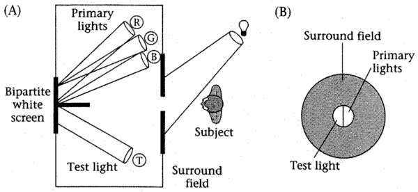
Color matching experiments. The basic color matching experiment is shown in the figure below:

The subject sees a white screen divided into two halves, one half illuminated by a test light, the other half illuminated by a mixture of one or more primary lights (here three are shown). The subject can adjust the intensity of the primary light(s) to try to make the two halves of the screen match.
Scotopic matching. Under low light conditions, called scotopic conditions, any test light can be matched by adjusting the intensity a single primary light. Physiologically, this is because under these conditions, only the retinal cells known as rods are involved, and these cells have only a single photopigment. Thus scotopic matching depends only on the spectral sensitivity of these cells (and the optical charcteristics of the rest of the experiment, of course). Thus we are mapping points in an N=31-dimenational space (lights with an arbitrary spectrum) onto a line (a 1-dimensional space).
In a scotopic color-matching experiment, we are manipulating two vectors -- the spectral power distributions of the test light (t) and the primary light (p) -- and a scalar -- the overall intensity adjustment of the primary light (e). Then when a primary light at intensity e subjectively matches a test light, we can say that t matches e*p. For a particular choice of primary p, the experiment then defines a function from vector t (the spectrum of the test light) to scalar e (the intensity of the primary light). We can write this as e = f(t) (though we might want to stick p in there somewhere, maybe in Octave-ese something like e = fp(t), where "fp" is just our name for the function that accomplishes the mapping we are interested in.
This function turns out to be linear -- it exhibits homogeneity and superposition.
Homogeneity: if t matches e*p, then a*t matches a*e*p (for an arbitrary scalar a); in other words, fp(a*t) = a*fp(t).
Superposition: if t matches e*p and t1 matches e1*p, then t+t1 matches e*p+e1*p. In other words, fp(t+t1) = f(t)+f(t1).
Since this function is linear, it must be equivalent to a matrix multiplication. That is, the mapping from the (n x 1) vector t to the (1 x 1) scalar e (for a given primary p) must be accomplished by a 1 x n "matrix" (i.e. a row vector) R, so that e = R*t
An equivalent statement is that e must be a linear combination (a weighted sum) of the elements of t. And another way to put it is that the equation -- like the eye -- projects an m-dimensional space (the spectrum of a light) onto a line (one dimension representing the perceived intensity of the light under scotopic conditions).
Furthermore, there are some obvious and simple ways to estimate what R is (there are some less obvious ways to solve such problems as well, but they will come later). The simplest is to test repeatedly with monochromatic test lights -- lights for which only one of the vector elements is non-zero. In this case, if it is the ith element of t that is non-zero, when we write out the full expansion of the equation e = R*t, we see that the right side reduces to the scalar product of the ith element of R times the ith element of t. This tells us that the ith element of R is just the slope of the line relating the intensity of the ith monochromatic test light intensity to the primary-light intensity, and this we can easily measure. Then all we have to do is to repeat the experiment 30 more times, with 30 other monochromatic lights, to get the full set of weights.
This also enables us to predict when two test lights t and u will match each other (under scotopic conditions): they will match if and only if R*t = R*u.
What about the matching functions for other primary lights (with different spectra)? Well, we know that (always under scotopic conditions) we can match an arbitrary new primary p1 with some scaling of our old primary p, such that p1 matches k*p.
It follows that if a*p matches a test light t, then a*k*p1 will also match t. From this it follows that the equivalent of R for p1 -- the matrix that expresses the color-matching function for the new primary light -- is just k*R. Thus across choices of primary light, R is unique up to a scale factor. Modulo this scaling effect, the elements of R are telling us how sensitive the eye is -- under scotopic conditions -- to the corresponding wavelengths of light.
Comparison to scotopic matching and rhodopsin absorption.
The apparatus shown in the figure below can be used to estimate the absorption spectrum of the rod photopigment rhodopsin.
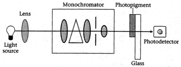
This tells us, for each monochromatic light, how much is absorbed. The result is a vector whose elements tell us how much of the corresponding wavelengths of light is absorbed.
If we compare the sensitivity of scotopic matching -- as measured in color-matching experiments by the scaling factor R -- to the absorption spectrum of the rod photopigment rhodopsin, we see a remarkable match. The graph below (from Wald and Brown 1956 via Wandell) shows a comparison between rhodopsin absorption (the filled circles) and scotopic sensitivity (the open circles):
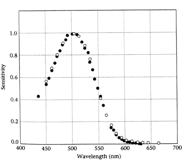
This is a striking example of harmony between psychophysics and physiology.
Photopic matching.
Under photopic conditions (where the cone cells are engaged), it takes intensity adjustment of three primary lights to match the appearance of an arbitrary test light. There is not a unique set of three primaries that we need for this purpose -- there are infinitely many possible sets of spectra that could serve effectively as primary lights. On the other hand, it is not just any three different lights with different spectra that will work.
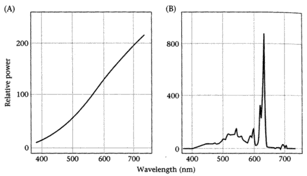
Scotopic vision sees just shades of grey, and photopic vision sees in color, but this does not mean that photopic vision sees color "as it is", i.e. in a way that makes lights equivalent just in case their spectra are the same. On the contrary, lights that are very different spectrally can look exactly the same to photopic vision. For instance, panel A of the figure below shows the spectral power distribution of a tungstun bulb, while panel B shows the spectral power distribution of the light from a television monitor that has been adjusted to match panel A.
Since photopic color-matching requires setting of three primaries, the quantities involved are the test light t (again an Nx1 vector), the three primary lights p1 p2 and p3 (each an Nx1 vector), and the three primary light settings e1 e2 and e3 (each a scalar). We can combine the three scalars e1 e2 e3 into a 3-element vector e. As before, a color-matching experiment (for a given set of primaries) is a function from a test light to a vector of primary-light settings: e = fp(t)
As before, we can test the color-matching experiment for linearity.
Superposition: if test light t is matched by primary settings e, and test light t1 is matched by primary settings e1, is test light t + t1 matched by primary settings e + e1 ? In fact it is. This fact about color matching is called Grassmann's additivity law, after Hermann Grassmann, a 19th-century high school teacher who also invented the earliest version of linear algebra and wrote the standard dictionary of Vedic Sanskrit.
We could also ask about homogeneity -- but actually, for the case of real numbers, superposition implies homogeneity. Therefore the photopic color-matching function fp() is linear, and can be represented as a matrix multiplication e = C*t ( in which t is an Nx1 column vector, C is a 3xN matrix, and e is a 3x1 column vector).
Note that (by the definition of matrix multiplication) this decomposes the problem into three versions of the scotopic function: the first element of e is the inner product of the first row of C and t ; the second element of e is the inner product of the second row of C and t ; and the third element of e is the inner product of the third row of C and t. The rows of the matrix C are sometimes called color-matching functions, because each of them can be seen as a set of coefficients that map a test light onto a setting for one of three primary lights.
Note also for a monochromatic test light (one in which only the ith component of t is non-zero), e will be exactly equal to the ith column of C times the ith element of t. Here is a simplified example with a 5-element test light in which just the third component is non-zero:
   C13t3     C11 C12 C13 C14 C15    0
   C23t3  =  C21 C22 C23 C24 C25    0
   C33t3     C31 C32 C33 C34 C35    t3
                                    0
                                    0
Thus we can figure out what C is in the same way that we figured out what R was in the scotopic case: by probing the system with n monochromatic lights, and looking in each case at the slope of the relationship between input intensity and output values. Each such estimate of the slope will give us one column of the matrix C.
All of this tells us that human color vision can be modeled as a three-dimensional subspace of the N-dimensional space of spectral power distributions. This is why lots of different primary lights will work: any set of three lights that span the three-dimensional subspace will work fine, and to a first approximation, this is any three lights whose spectral power distributions are linearly independent.
There is an important caveat. We can't have negative lights: we can multiply a light by scalars from zero on up, but multiplication by a negative number is not physically realizable. This means that for any set of primary lights, there will in fact always be some test lights that can't be matched, because matching them would require a negative setting of one or two of the primaries. To accomplish this within the physical constraints, we need to make the experimental apparatus a bit more complicated, so that we can move one or two of the primary lights over to the test-light side -- since this is equivalent to scaling them by a negative number on the primary-light side. See Wandell's chapter for more details if you care about the psychophysics as well as the linear algebra.
Color-matching functions for different set of primary lights.
Suppose we determine the system matrix (the matrix whose rows are the color-matching functions) for two different sets of primary lights. How do we relate the two systems?
Since we think of each light's spectral power distribution as a column vector, it's convenient to represent a set of three lights as an Nx3 matrix P whose three columns are the vectors for the three lights. Then the light resulting from a setting of primary intensities e will be P*e, that is, an Nx1 vector of the spectral intensities that result from scaling each primary by its element of e, and adding up the results.
We know that two lights t and t1 will match each other just in case each matches the same setting of a given set of primaries. For color-matching matrix C (defined for any set of primary lights), this means that Ct = C*t1 . Thus the light resulting from a given setting e of primaries P (that is, P*e) will match a test light t iff C*t = C*P*e.
Now we match the same test light to a different set of primaries P1, giving a new set of intensities e1.
The resulting light P1*e1 also matches t, so we know that C*t = C*P1*e1. (This is still the color-matching matrix C from the old primaries P -- it doesn't matter, because P1*e1 is still just a light, so if it matches t then we know t and P1*e1 must be projected onto the same e by C.
Since C*t = C*P*e and C*t = C*P1*e1, it follows that C*P*e = C*P1*e1 . Multiplying both sides on the left by (C*P)^-1, we find that
e = ((C*P)^-1) *C1*e1
This equation gives a way to predict the mapping from the "knob settings" for one set of primaries to the "knob settings" for another, as long as we also know the spectral composition of the two sets of primaries (P and P1), and some color matching matrix C (which need not come from either set of primaries!)
We can express this relationship more succinctly as e = M*e1 , where M is a 3 x 3 matrix that equals ((C*P)^-1)C*P1*e1
This equation can in principle be quite a useful one, since it allows us (for instance) to create matching colors on CRTs with different phosphors, or color printers with different basic inks. The details of actual applications are these principles can be complicated, but this relationship provides the fundamental reason why it's possible to reproduce color images using a variety of limited sets of color primitives (phosphors, inks etc.) that may give quite different basic color impressions.
New color-matching matrices from old
We have a set of primaries P with associated color-matching matrix C. Given a new set of primaries P1, how can we determine the associated color-matching matrix C1 ?
The spectrum of the mixture of primaries P1 that matches any light t will be P1*C1*t . (We don't know what C1 is yet, but just wait, we're going to derive it...)
If we treat this as a test light, the matching mixture of primaries P will be C times it, i.e. C*P1*C1*t
This will be the same as the mixture of primaries P that matches t (i.e. C*t), by construction, so
C*P1*C1*t = C*t
Multiplying both sides on the left by inv(C*P1), we get
C1*t = inv(C*P1))*C*t
This shows that inv(C*P1)*C (i.e. the inverse of CP1 times C) has the same effect on t that C1 does.
This doesn't show that it's the same as C1 -- but it's good enough for our purposes.
Relationship to the underlying physiology.
As in the case of scotopic vision, the photopic color-matching function can be related to the absorption spectra of the photopigments that are the basic sensory mechanism in vision. The basically three-dimensional character of color vision comes from the fact that there are three different photopigments in the cone cells in the retina.
According to Wandell, "the best estimates of the cone photopigment absorptions are derived from measurements of the cone photocurrent, that is, the change in the current flow through the membrane of individual cones are they are stimulated by light." Note that this is not yet a neuronal signal: that is, we are still looking at the physiology of a sensory cell, and have not yet passed the first synapse into the nervous system itself, where information is primarily encoded by neuron firing rates. Even so, the cone cell membrane current is not a linear function of light input.
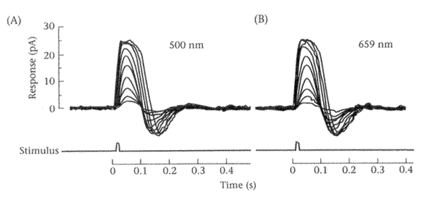
The figure above shows responses of a single (type of?) cone cell to brief monochromatic flashes of various strengths at the wavelengths indicated. How can we tell that the response is not linear? There are two basic indicators:
Why then is the psychophysics of color matching so beautifully linear?
This "why" question has two meanings: a causal why: how does the nervous system accomplish it? and a teleological why: why has evolution arranged for the nervous system to accomplish it?
There is a simple answer to the second question: light mixing is linear, and therefore is it useful for the perception of light mixing to be linear as well. There is more to say about this, but we can leave it there for now.
There is also a fairly simple answer to the first question, but it is harder to understand. Light absorption by photopigments is linear. The cell membrane response is non-linear, but it is a static non-linearity: it is independent of the initial linear encoding process (i.e. it only depends on the output of that process). In this case, it is easy to characterize the overall system, and certain ways of looking at it will show linear behavior.
The figure below shows peak photocurrents for a (type of?) cone cell stimulated by different magnitudes of two different monochromatic lights. Each of the curves shows a highly non-linear relationship between stimulus level and response level -- it is clear that scaling the input does not scale the output! We can see the saturation effect at higher input levels, and also a threshold effect at lower input levels.
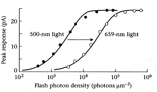
However, we can look at the two curves in a different way: what relative intensities of the 500-nm and 659-nm lights will give the same peak photocurrent response? We do this by picking a y-axis (response) level, and looking at the points of intersection with the two curves. When we look at them this way, we can see that the 659-nm curve is almost exactly the 500-nm curve shifted over by a constant amount. Since the x-axis is a log scale, this means that the constant-response light intensities are related by a constant ratio -- and this means that homogeneity will be satisfied in color-matching at the photocurrent level!
Comparisons of this type can be used to establish (from the cone photocurrents) the underlying cone photopigment sensitivities:
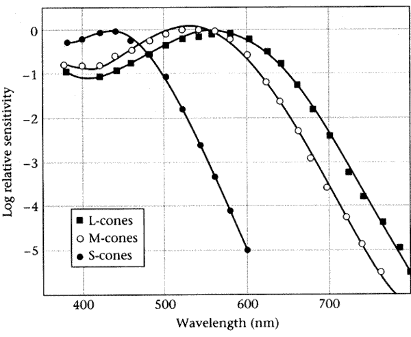
See Wandell's explanation for more details on how this is done. For us, this particular analysis is much less important than the general point: certain types of non-linear system (those in which a static nonlinearity follows a linear stage) may nevertheless behave linearly when we look at certain relationships among system responses to different inputs, rather than at the system response to a single input. Wandell presents the following analysis for a single cone type. It should be clear how it generalizes to deal with all three cone types.
There is a photopigment system matrix ... A that maps the test light into a photon absorption rate At. Second, the static nonlinearity converts [this] into a peak phocurrent response ... F(At).
When we set a match between the peak photocurrent from the test light and the primary light, we establish an equation of the form
F(At) = F(aAp)
where a is the intensity of the primary light needed to match the test light. Since the non-linear function F is monotonic, we can remove it from both sides of the equation and write
At = aAp
From this equation, we see that there is a linear relationship between the primary- and test-light intensities, since if t matches ap, then kt will match kap.
It's worth reading Wandell's section "Why this is a big deal." Some highlights:
We should remember that the relationship between behavior and biology may not always be found at the level of the measurements that are natural within each discipline...
... [Y]ou may be tempted to interpret a physiological measurement as a direct predictor of some percept. The rate a which a neuron responds and the stimulus that excites a neuron powerfully are natural biological measures. Remember, however, that there is no simple relationship between the photocurrent response and the intensity level of primary light. We achieved a good link between the physiological and behavioral measures by structuring a theory of the information that is preserved in each set of experimental measurements. Understanding our measurements in terms of this level of abstraction -- what information is present in the signal -- is a harder but better way to forge links between different disciplines.