In this segment, we will be dealing with the properties of sequences made up of integer powers of some complex number:
x[n] = z^n for n from -infinity to infinity, z some complex number
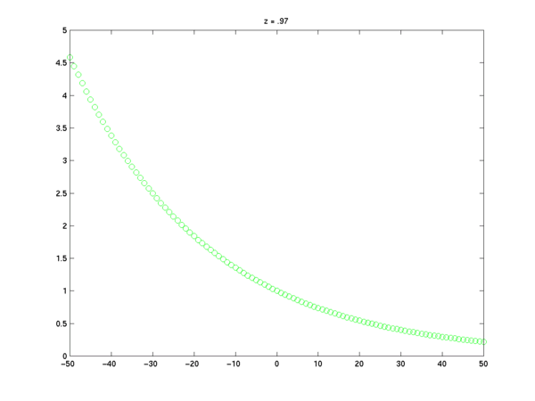
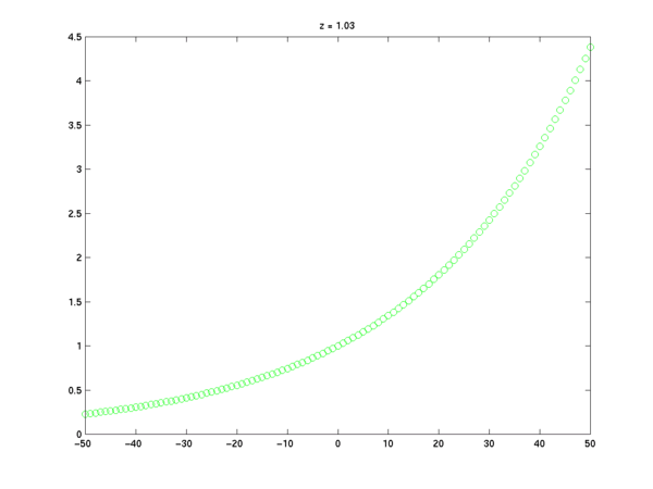
You should start with a clear graphical intuition about what such sequences are like. If the number z happens to be one or zero, we will get a sequence of constant values. If z is a positive real number, we will get a sampled exponential ramp, that is either rising or falling depending on whether z is less than 1 or greater than 1:
n = -50:50;
z = .97;
x = z.^n;
plot(n,x,'go'); title('z = .97');

z = 1.03;
x = z.^n;
plot(n,x,'go'); title('z = 1.03');
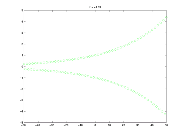
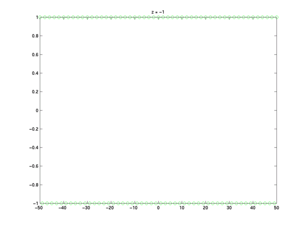
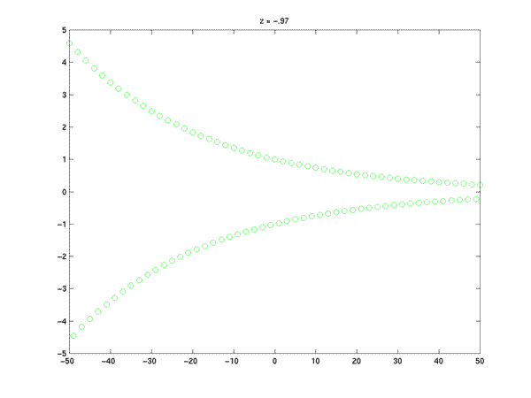
If the number z is a negative real number, we will get a sequence that alternates between positive and negative values. Depending on whether z is less than, equal to, or greater than -1, these values will increase exponentially, remain constant, or decrease exponentially in magnitude with increasing n.
z = -1.03; x = z.^n; plot(n,x,'go'); title('z = -1.03');
z = -1; x = z.^n; plot(n,x,'go'); title('z = -1');
z = -.97; x = z.^n; plot(n,x,'go'); title('z = -.97');
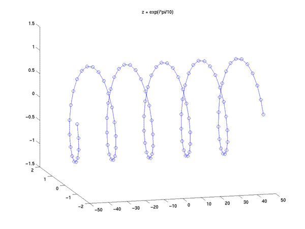
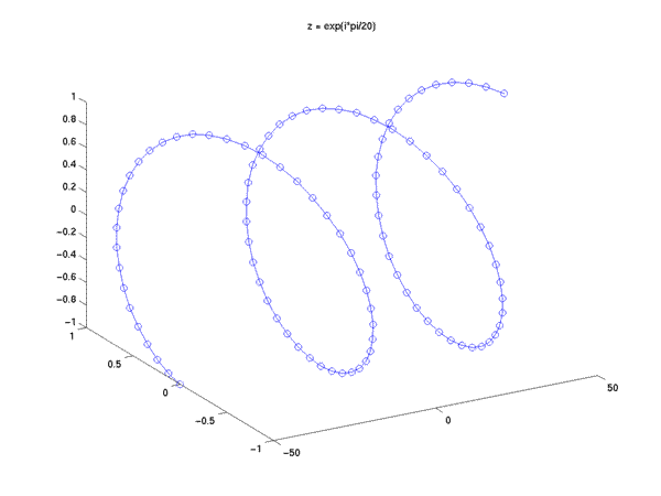
If z is a complex number that happens to lie on the unit circle (in the complex plane, with the x-axis representing the real part of z and the y-axis representing the imaginary part), then z^n will be a sinusoid sampled at intervals of angle(z) radians.
This can easily be shown by considering that in this case z = e^(i*w) for some real number w, which is equivalent to cos(w) + i*sin(w), so that z^n will be e^(i*n*w), or cos(n*w) + i*sin(n*w).
z = exp(i*pi/10); x = z.^n;
plot3(n, real(x), imag(x), 'o');
hold on;
plot3(n, real(x), imag(x), '-');
title('z = exp(i*pi/10)');
hold off; view(-15,15);
z = exp(i*pi/20); x = z.^n;
plot3(n, real(x), imag(x), 'o');
hold on;
plot3(n, real(x), imag(x), '-');
title('z = exp(i*pi/20)');
hold off; view(-30,30);
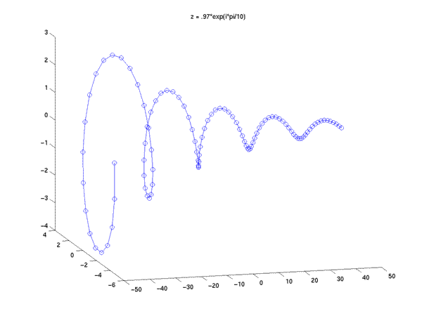
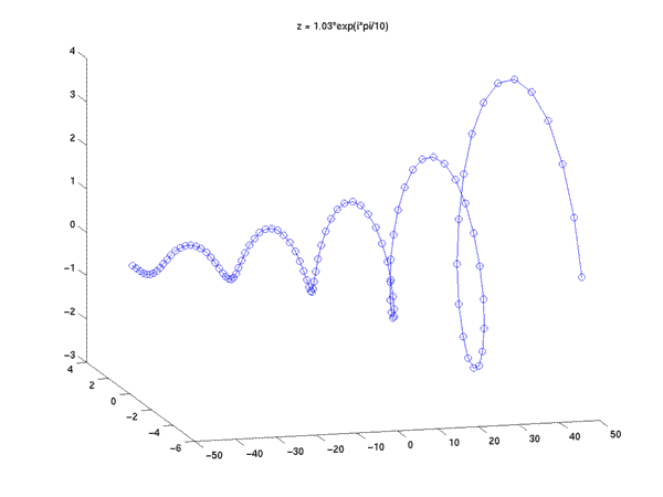
If z is a complex number (with a non-zero imaginary part) whose magnitude is slightly less than or greater than 1, then z^n will be a sinusoidal spiral like those we have just seen, whose magnitude is exponentially decreasing or increasing depending on whether z has a magnitude less than or greater than 1.
z = .97*exp(i*pi/10); x = z.^n;
plot3(n, real(x), imag(x), 'o');
hold on;
plot3(n, real(x), imag(x), '-');
title('z = .97*exp(i*pi/10)');
hold off; view(-15,15);
z = 1.03*exp(i*pi/10); x = z.^n;
plot3(n, real(x), imag(x), 'o');
hold on;
plot3(n, real(x), imag(x), '-');
title('z = 1.03*exp(i*pi/10)');
hold off; view(-15,15);
Now suppose a linear time-invariant (LTI) system with impulse response h(n) has as its input one of these exponential sequences
$$x[n] = z^n$$
for some (arbitrarily chosen) complex number z.
The output will be the convolution sum h # x, or
$$y[n] = \sum_k h[k] x[n-k] \\
= \sum_k h[k] z^{n-k} \\
= z^n \sum_k h[k] z^{-k}
$$
Thus the input was \(z^n\), and the output is \(z^n\) multiplied by a constant that depends on the value of z and on the impulse response h. If we write that constant as
$$H(z) = \sum_{k} h[k] z^{-k}$$
then we can rewrite the system equation as
$$y[n] = H(z) z^n$$
We can see another way to say this if we express the LTI system with impulse response h in the more general form of the "convolution matrix" \(M_h\) -- that is, a matrix with a set of shifted time-reversed copies of the impulse response h in its rows, as discussed in an earlier lecture. Now since
$$y[n] = M_h z^n = H(z) z^n$$
we can see that the complex exponential \(z^n\) is an eigenvector of \(M_h\), with \(H(z)\) as the eigenvalue, since \(M_h\) times \(z^n \)equals the constant \(H(z)\) times \(z^n\).
Because of the superposition property of linear systems, this "eigenrelationship" makes it convenient to express a signal as a linear combination of complex exponentials. If
$$x[n] = \sum_k a_k z_k^n$$
then the system output for an LTI system with impulse response h will be
$$y[n] = \sum_{k} a_k H(z_k) z_k^n$$
That is, the output is also a linear combination of the same set of complex exponential sequences, with each coefficient being the product of the input coefficient \(a_k\) and the system's eigenvalue \(H(z_k)\) for the eigenfunction \(z_k^n\).
The expression for the system eigenvalues in terms of z is known as the "z transform" of h (for n from -infinity to infinity):

The z-transform equation is closely related to that for the DFT. There's a crucial practical difference, in that we literally perform Discrete Fourier Transforms on concrete input vectors to produce concrete output vectors. We can't do that with the z transform, since (given a sampled impulse response) it defines a function on all points in the complex plane, so that both inputs and outputs are drawn from continuously infinite sets.
Nevertheless, the z transform has an enormous -- though indirect -- practical value. As we'll soon see, we can use it to perform a valuable analysis of an arbitrary linear constant-coefficient difference equation, deriving an expression for the z transform of the system's impulse response which we can use to calculate the system's "poles" and "zeros" in the frequency domain.
Recall that the DFT is
$$X(k) = \sum_{n} x[n] e^{-i(2\pi/N)kn}$$
If we rewrite the exponential on the right hand side slightly as
$$(e^{ik(2\pi/N)})^{-n}$$
each value of k can be seen as just picking a different complex number$$z = exp(i k 2 \pi/N)$$
to serve as the basis for a complex exponential series.
However, a better analogy for the z transform is the DTFT, not the DFT.
Remember that the DFT relates
x[n], a periodic function of a discrete variable x in the time domain, to
X[k], a periodic function of a discrete variable k in the frequency domain.
The "discrete time fourier transform" (DTFT) relates
x[n], a nonperiodic function of a discrete variable x in the time domain, to
X(w), a periodic function of a continuous variable w in the frequency domain.
As a result, the DTFT shares with the z-transform the fact that the transform equation defines a function of a continuous (complex) variable, and that the input side of the equation sums over all n rather than a finite set:
DTFT:
$$X(w) = \sum_{n=-\inf}^{\inf} x[n] e^{-iwn}\\
= \sum_{n=-\inf}^{\inf} x[n] (e^{iw})^{-n}$$
Since \(e^(ix) = cos(x) + i sin(x)\), restricting z to imaginary powers of e is the same as requiring that abs(z) = 1, i.e. that (in the complex plane) z must fall on a circle with radius one.
We can look at this another way. Let's express the complex number z in polar form as \(r e^{iw}\). Then the z-transform of \(x[n] \)
becomes
$$X(re^{iw}) = \sum_n x[n] (re^{iw})^{-n}$$
or
$$X(re^{iw}) = \sum_n x[n] r^{-n} e^{-iwn}$$
The right-hand side of this equation is just the DTFT of the sequence x[n] multiplied by a real exponential \(r^{-n}\). Thus
$$X(re^{iw}) = X(z) = DTFT(x[n]r^{-n})$$
where r is the magnitude of z. Where r = 1, X(z) = DTFT(x).
The z transform is unusual, in being named after a letter of the alphabet rather than a famous mathematician. The Fourier transform is named after Baron Jean Baptiste Joseph Fourier (1768-1830); the Walsh-Hadamard transform is named after J.L. Walsh (?) and Jacques Salomon Hadamard (1865-1963); we haven't discussed the Laplace and Hilbert transforms yet, but we will (at least briefly), and they are named after Pierre-Simon de Laplace (1749-1827) and David Hilbert (1862-1943) respectively.
Laplace transforms have long been used in solving (continuous-time) linear constant-coefficient differential equations.
According to p 420 of Contemporary Linear Systems (Strum and Kirk 1994),
A method for solving linear, constant-coefficient difference equations by Laplace transforms was introduced to graduate engineering students by Gardner and Barnes in the early 1940s. They applied their procedure, which was based on jump functions, to ladder networks, transmission lines, and applications involving Bessel functions. This approach is quite complicated and in a separate attempt to simplify matters, a transform of a sampled signal or sequence was defined in 1947 by W. Hurewicz as
which was later denoted in 1952 as a "z transform" by a sampled-data control group at Columbia University led by professor John R. Raggazini and including L.A. Zadeh, E.I. jury, R.E. Kalman, J.E. Bertram, B. Friedland, and G.F. Franklin.
The Hurewicz equation is not expressed in the same way as the z transform we have introduced -- it is one-sided, and it is expressed as a function of the sampled data sequence f rather than the complex number z -- but the relationship is clear, and the applications were similar from the beginning. So perhaps the z transform should really be called the "Hurewicz transform" -- but it is too late to change.
In any case, it is presumably not an accident that the z transform was invented at about the same time as digital computers.
Consider \(x[n] = a^n u[n]\). Its z-transform is
$$X(z) = \sum_{n=-\inf}^{\inf} a^n u[n] z^{-n} \\ = \sum_{n=0}^{\inf} (a z^{-1})^n$$
This will converge (the sum will be finite) just in case
abs(z) > abs(a)
Since for any geometric series
$$\sum_{n=0}^{\inf} c r^n = c/(1-r)$$
the z-transform sum above will be
$$ X(z) = 1/(1-a/z) = z/(z-a) \;\;\; |z| > |a| $$
This equation for the z-transform of \(x[n] = a^n u[n]\)
$$X(z) = z/(z-a)$$
is a "rational function", that is, a ratio of polynomials. We can characterize it by its zeros (the roots of the numerator) and its poles (the roots of the denominator).
In this case there is one zero (z = 0) and one pole (z=a).
We also need to know the "region of convergence" (ROC) for the z-transform (here |z| < |a|). For the next section of exposition, we will neglect the ROC. This is not a good idea in general.
It follows directly from the definition
$$X(z) = \sum_{n} x[n] z^{-n}$$
that the z-transform is LINEAR: that is, if
$$x[n] = c x1[n]$$
then
$$X(z) = \sum_n c x1[n] z^{-n} = c \sum_n x1[n] z^{-n} = c X1(z)$$
and if \(x[n] = x1[n] + x2[n]\) then
$$ X(z) = \sum_n (x1[n] + x2[n]) z^{-n}\\ = \sum_n x1[n] z^{-n} + \sum_n x2[n] z^{-n}\\ = X1(z) + X2(z) $$
Thus if
$$x[n] = a^n u[n] + b^n u[n]$$
then
$$X(z) = z/(z-a) + z/(z-b) \\ = \frac{z(z-b) + z(z-a)}{(z-a)(z-b)} \\ = \frac{z(2z-(b+a))}{ (z-a)(z-b)}$$
In addition to linearity, z-transforms have a number of other properties that make them a useful tool in analyzing LTI systems:
As with the special case of the Fourier transform, convolution in the time domain is multiplication in the z domain:
If \(\;\;x[n] = x1[n] * x2[n]\)
then \(\;\;X(z) = X1(z) X2(z)\)
(where '*' is interpreted as a binary convolution operator).
If \(\;\;x[n] = x1[n-k]\)
then \(\;\;X(z) = z^{-k} X1(z)\)
If \(\;\;x[n] = x1[-n]\)
then \(\;\;X(z) = X1(1/z)\)
The convolution property of the z-transform means that for an arbitrary LTI system with impulse response h[n], the system equation
\(y[n] = h[n] * x[n] \)
implies that
\(Y(z) = H(z) X(z)\)
and therefore
\( H(z) = Y(z)/X(z) \)
We can also express the same LTI system as a linear constant-coefficient difference equation, if the system is causal:
$$\;\;\;\;\;a_0 y[n] + a_1 y[n-1] + ... + a_M y[n-M] \\ = b_0 x[n] + b_1 x[n-1] + ... + b_N x[n-N]$$
If this concept is not entirely clear to you, you may want to review the lecture notes on Digital Filters as Linear Constant-Coefficient Difference Equations.
We can take the z-transform of both sides of the above equation, representing the z-transform by the notation Z{...}.
$$\;\;\;\;\;Z\{ a_0 y[n] + a_1 y[n-1] + ... + a_M y[n-M] \} \\ = Z\{ b_0 x[n] + b_1 x[n-1] + ... + b_N x[n-N] \}$$
Since the z-transform is linear, we can take it term-wise:
$$\;\;\;\;\;Z\{ a_0 y[n] \} + Z\{ a_1 y[n-1] \} + ... + Z\{ a_M y[n-M] \} \\ = Z\{ b_0 x[n] \} + Z\{ b_1 x[n-1] \} + ... + Z\{ b_N x[n-N] \}$$
Likewise we can pull the b and a constants outside each transformed term:
$$\;\;\;\;\;a_0 Z\{ y[n] \} + a_1 Z\{ y[n-1] \} + ... + a_M Z\{ y[n-M] \} \\ = b_0 Z\{ x[n] \} + b_1 Z\{ x[n-1] \} + ... + b_N Z\{ x[n-N] \}$$
Now the shift property of the z-transform lets us replace (for all k)
\(Z\{x[n-k]\}\) with \(z^{(-k)} Z\{x[n]\}\) and
\(Z\{y[n-k]\}\) with \(z^{(-k)} Z\{y[n]\}\) :
$$\;\;\;\;\;a_0 Z\{ y[n] \} + a_1 z^{(-1)} Z\{ y[n] \} + ... + a_M z^{(-M)} Z\{ y[n] \} \\ = b_0 Z\{ x[n] \} + b_1 z^{(-1)} Z\{ x[n] \} + ... + b_N z^{(-N)} Z\{ x[n] \}$$
Now all the Z{...} expressions are either \(Z\{x[n]\}\) or \(Z\{y[n]\}\)
and so we can replace them all with \(X(z)\) or \(Y(z)\):
$$\;\;\;\;\;a_0 Y(z) + a_1 z^{(-1)} Y(z) + ... + a_M z^{(-M)} Y(z) \\ = b_0 X(z) + b_1 z^{(-1)} X(z) + ... + b_N z^{(-N)} X(z)$$
Factoring out Y(z) and X(z):
$$\;\;\;\;\;Y(z) ( a_0 + a_1 z^{(-1)} + ... + a_M z^{(-M)} ) = X(z) ( b_0 + b_1 z^{(-1)} + ... + b_N z^{(-N)} )$$
The convolution property of the z-transform told us that H(z), the z-transform of the system's impulse response, is equal to Y(z)/X(z), so let's solve for Y(z)/X(z) in our equation:
$$\;\;\;\;\;\frac{Y(z)}{X(z)} = \frac{b_0 + b_1 z^{(-1)} + ... + b_N z^{(-N)}}{a_0 + a_1 z^{(-1)} + ... + a_M z^{(-M)}}$$
By convention, \(a_0\) is 1. We can multiply through by \(1/b_0\), replacing the b coefficients with c coefficients such that \(c_n = b_n/b_0\):
$$\frac{Y(z)}{X(z)} = \frac{1}{b_0} \frac{1 + c_1 z^{(-1)} + ... + c_N z^{(-N)}}{ 1 + a_1 z^{(-1)} + ... + a_M z^{(-M)} }$$
If a_0 is already 1, then the c coefficients are just the same as the b coefficients.
Thus the z-transform of the impulse response of such a system--- ANY system described by a linear constant-coefficient difference equation--- is a ratio of polynomials in z^(-1), where the coefficients in the numerator come from the x (input) coefficients in the difference equation, and the coefficients in the denominator come from the y (output) coefficients in the difference equation.
Let's go back to our expression for H(z):
$$\frac{Y(z)}{X(z)} = \frac{1}{b_0} \frac{1 + c_1 z^{(-1)} + ... + c_N z^{(-N)}}{ 1 + a_1 z^{(-1)} + ... + a_M z^{(-M)} }$$
The fundamental theorem of algebra tells us that we can express the numerator and denominator polynomials uniquely as a product of first order terms in \(z^{(-1)} = 1/z\), with (complex) coefficients \(q_1, ..., q_N\) and \(p_1, ..., p_M\):
$$H(z) = \frac{1}{b_0} \frac{(1 - \frac{q_1}{z} ) (1 - \frac{q_2}{z}) ... (1 - \frac{q_N}{z})} {(1 - \frac{p_1}{z} ) (1 - \frac{p_2}{z}) ... (1 - \frac{p_M}{z}) }$$
In this equation, each of the \(q_n\) and \(p_n\) is a complex number. If z equals one of the \(q_n\), the numerator becomes zero, and so does the whole function H(z). These values are called "zeros" of the system. As z approaches one of the \(p_n\), the denominator approaches zero, and the value of the function H(z) approaches infinity. These values are called "poles" of the system; graphically, you can imagine putting the complex plane on the ground, so that a pole sticks up into the sky at the point where z = \(p_n\).
Starting with our original linear constant-coefficient difference equation
$$\;\;\;\;\;a_0 y[n] + a_1 y[n-1] + ... + a_M y[n-M] \\ = b_0 x[n] + b_1 x[n-1] + ... + b_N x[n-N]$$
we have given a mechanical procedure for deriving an expression for the (factored form of the) Z transform of the system impulse resonse h[n]:
$$H(z) = \frac{1}{b_0} \frac{(1 - \frac{q_1}{z} ) (1 - \frac{q_2}{z}) ... (1 - \frac{q_N}{z}) }{ (1 - \frac{p_1}{z} ) (1 - \frac{p_2}{z}) ... (1 - \frac{p_M}{z}) }$$
If all of the "a" coefficients are zero, then the output is just a moving weighted average of the input, and the denominator of our expression for H(z) will be 1. This is a filter with only zeros and no poles, an "all-zero" filter.
Conversely, if all of the "b" coefficients are 0 (except of course for \(b_0\) which must be 1, or the system would ignore the input!), then the current output sample is basically predicted as a weighted combination of the earlier output samples, and the numerator of our expression for H(z) will be 1. This is a filter with only poles and no zeros, an "all-pole" filter.
If the difference equation has both "a" and "b" coefficients, then the filter has both poles and zeros.
Some important properties of poles and zeros follow from this algebraic background. For example, if we are dealing with real-valued signals -- as we normally are -- than the coefficients of the LCCDE must obviously also be real. It follows that the roots of the numerator and denominator polynomials in the z-transform will either be real, or will come in complex-conjugate pairs. Thus the zeros and poles will likewise either be real, or will come in complex-conjugate pairs, since they are just the roots of the numerator and denominator polynomials.
This part is easy -- given a computer program to do the calculations -- because it is just a matter of factoring or expanding polynomials. In Matlab, the function roots() will take us from polynomial coefficients to the roots of the polynomial, while poly() will take us from the roots back to the polynomial coefficients. The a or b coefficients (such as are used in filter()) are polynomial coefficients.
Thus if p is a vector containing the z-values of the poles of a system (the roots of the denominator polynomial in its z-transform), then the a coefficients will be a = poly(p), while we can go the other way with p = roots(a). Likewise for the zeros (the roots of the numerator polynomial).
See the next section for a concrete example.
Since we know that the z-transform reduces to the DTFT for \(z = e^{iw}\), and we know how to calculate the z-transform of any causal LTI (i.e. the z-transform of its impulse response) from the coefficients of the difference equation, we can write down an expression for its spectrum (i.e. the ratio of the spectrum of the output to the spectrum of the input) by simply setting \(z = e^{iw}\) in the z-transform.
This expression will be a periodic, continuous function of the variable w, which is frequency in radians. The period is obviously 2pi. We can get N evenly-spaced samples of one period of the spectrum (which is also what the DFT gives us) by setting (in Matlab-ish) w to (n/N)*2*pi for n = 0 to N-1, i.e. \(z = e^{i(n/N)2\pi} \) for n = 0 to N-1.
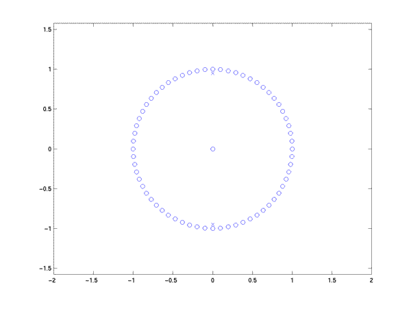
This is quite easy to calculate. It is also especially easy to think about graphically, if we represent the system in pole-zero form:
>> circle = exp(i*(0:63)*2*pi/64); # 64 points around the unit circle
>> plot(real(circle),imag(circle),'o');
>> r = .95*exp(i*.5*pi);  # complex root at frequency .5, amplitude .95
>> axis([-2 2 -2 2]); axis('equal'); hold on
>> plot(real(r),imag(r),'bx', real(r'),imag(r'),'bx'); # plot complex conjugate poles
>> plot(0,0,'bo'); # plot zero
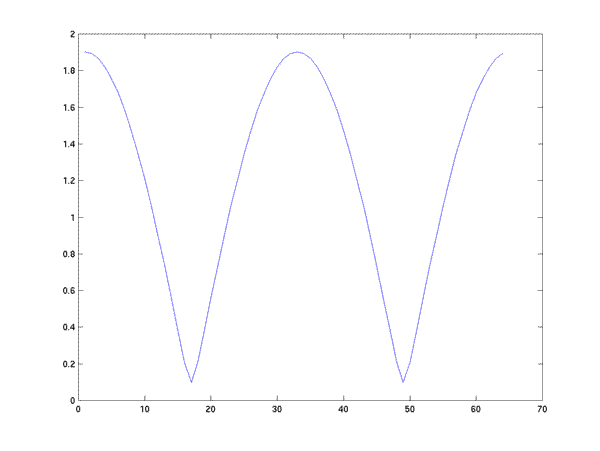
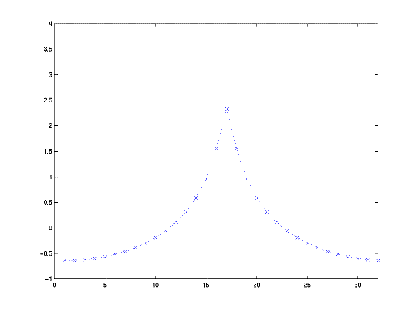
Now we just evaluate the factored form of the z-transform of a system with these poles (and the single, necessary, degenerate zero). This is the product of the differences between the z-values (here the points on the unit circle) and the roots r and r'. The sampled spectrum is just the inverse of this product of distances:
>> distances = (abs(circle-r) .* abs(circle-r'));
>> plot(distances);
>> plot(1:64,log(1./distances),'bx:');
>> axis([0 32 -1 4]);
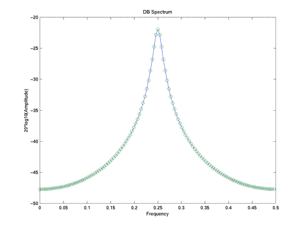
Of course, an alternative method of calculation -- generally simpler in practice -- is simply to take the DFT of the impulse response of the filter.
>> A=poly([r r'])
A =
    1.0000   -0.0000    0.9025
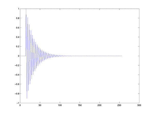
>> impulse=zeros(256,1); impulse(15)=1;
>> impresp = filter([1 0 0],A,impulse);
>> plot(impresp);
>> lspecplot(fft(impresp),1);
[TK]
We've mentioned that the recursive part of the LCCDE filter -- the output side, which contributes the a coefficients -- is sometimes called an autoregressive filter. It expresses each sample as a linear combination of \(N_a\) previous samples, and we can think of this as being like predicting each sample in the sequence by linear regression on the previous \(N_a\) samples.
Suppose we are given a signal that was actually generated by such an autoregressive filter -- one in which all the b coefficients except for \(b_0\) are 0. Will each sample actually be exactly the inner product of the filter's a coefficients with the \(N_a\) previous samples? No, not exactly, because the input to the system will still have an effect, being fed in through the \(b_0\) coefficient. However, for many combinations of inputs and system values, we will still be able to estimate the a coefficients in a useful way. One ubiquitous method of speech analysis -- linear predictive coding, or LPC -- is based on this assumption.
Assume that within some (fairly short) region of speech, M samples long, we are predicting each sample as a linear combination of N previous samples, i.e.$$p(i) = \sum_j a(j) s(i-j)\;, \;\;\;1 <= j <= N, \;\;\;\;N <= i < M$$
In matrix notation,
$$p = S a$$
where p is an M X 1 matrix (column vector) of predicted values, S is an M X N matrix whose ith row contains speech samples s(i) to s(i+N-1), and a is an N X 1 matrix (column vector) of prediction weights.
Thus for a third-order predictor, with input samples s1 ... sM and predictor coefficients [a(1) a(2) a(3)], p = S a means
 p(4)    =    s(1) s(2) s(3)     X     a(1)
 p(5)         s(2) s(3) s(4)           a(2)
 p(6)         s(3) s(4) s(5)           a(3)
 p(7)         s(4) s(5) s(6)
  .            .    .    .
  .            .    .    .
  .            .    .    .
 p(M)         s(M-3) s(M-2) s(M-1)
Notice that this is closely related to the previously-discussed concept of a recursive filter, and exemplifies why such filters are commonly called "autoregressive".
In this case, the a(i) are just the coefficients of the left-hand (output) side of a linear constant-coefficient difference equation--- ignoring the a(0) coefficient in of an LDCE, which is 1 by convention.
We know "S" in "p = S a," but not "a" or "p". What should we do? Suppose that we want to choose the weights "a" so as to minimize the prediction error
norm(S*a - s)
This is what is called a "least squares" problem: find a vector x providing the "best" solution to an overdetermined system of equations Ax = b, where "best" means "minimizing norm(Ax-b)".
There are a variety of methods of solving such problems, depending on the properties of A and b. MATLAB offers us two solutions, x = A\b and x = pinv(A)*b. We've seen the "backslash" A\b solution before; we'll discuss the pseudoinverse solution pinv(A)*b at greater length later.
For now, we'll just observe that if A has more rows than columns and is not of full rank, then "choose x to minimize norm(A*x - b )" does not have a unique solution. The solution x = pinv(A)*b give us the smallest x (x minimizing norm(x)) while the solution x = A\b gives the x with the fewest possible nonzero components.We'll examine the this question as we come to it in practice, but if there is a difference, the pseudo-inverse solution is probably the one that we want.
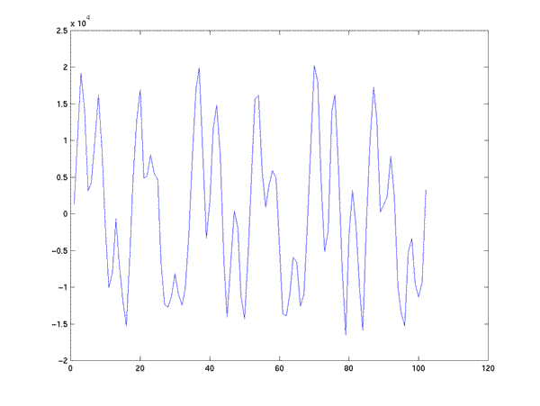
Let's get a chunk of speech to work with:
>> load('audio1');
>> S1 = S(2246:2347);
>> plot(S1);
>> length(S1)
ans =
   102
This is just a convenient piece of the middle of a vowel from the audio file we have used before. It represents as close to 3 pitch periods as we can get in this sampled signal:
Now let's get things set up as specified.
If we had a vector of input samples [1 2 3 4 5 6 7 8 10], and we were going to construct a third-order predictor, and we wanted to avoid making hypotheses about samples outside the range of input samples we would need A x = b to come out as
        A         x      b

        1 2 3  *  x1  =  4
        2 3 4     x2     5
        3 4 5     x3     6
        4 5 6            7
        5 6 7            8
        6 7 8            9
        7 8 9            10
In this situation, A is pretty close to what is called a "Hankel" matrix (see "help hankel" in Matlab), and so we can get A set up by
 function A = makeA(S,N)
 %
 % Set up matrix for linear prediction calculation
 % S is a vector of length M whose ith sample will be predicted
 % as a linear combination of the N previous samples.
 % Thus we want to set up a matrix A,
 % with M-N rows and N columns,
 % whose jth row consists of the samples from S(j) to S(j+N-1).
 % Obviously M must be greater than N.
 AA = hankel(S,S(1:N));
 A = AA(1:(length(S)-N),:);
Thus we get
>> makeA(1:10,3)
ans =
     1     2     3
     2     3     4
     3     4     5
     4     5     6
     5     6     7
     6     7     8
     7     8     9
The role of b in our equation Ax=b will be played by the input samples from S(N+1) to S(M).
>> A = makeA(S1, 14);
>> b = S1(15:length(S1));
A is full rank
>> rank(A)
ans =
    14
and so it doesn't matter much what method we use to get x:
>> norm(A\b - pinv(A)*b)
ans =
   5.0799e-15

>> x = pinv(A)*b;
>> x'
ans =
  Columns 1 through 7
   -0.1660    0.3545   -0.4917    0.5188   -0.7772    1.0481   -1.3567
  Columns 8 through 14
    1.1888   -1.5503    1.4317   -1.0071    0.8159   -1.2254    1.4033
How much of the variance of the input have we accounted for?
>> sum((A*x-mean(A*x)).^2) / sum((b-mean(b)).^2)
ans =
    0.9294
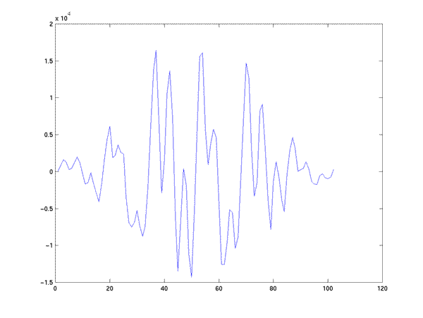
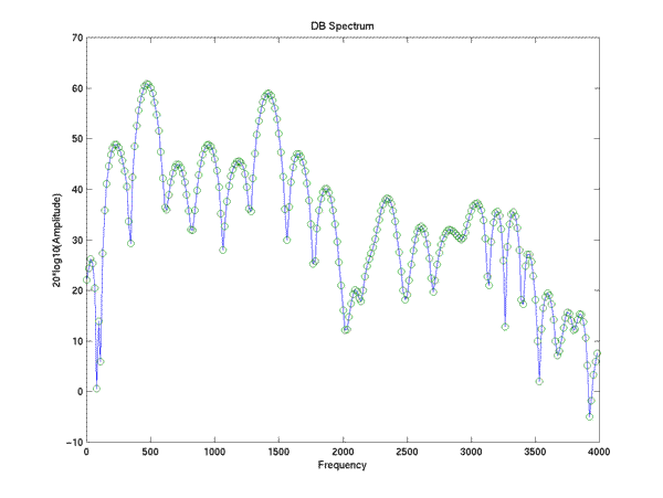
Let's look at the (windowed version of the) original signal, and its DFT spectrum:
>> S2 = hamming(length(S1)).*S1;
>> plot(S2);
>> q = zeros(512,1);
>> q(1:length(S2)) = S2;
>> lspecplot(fft(q), 8000);
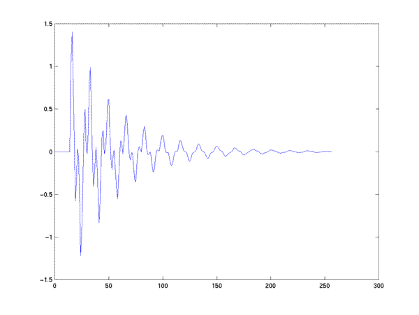
Now let's look at the impulse response of the recursive filter whose coefficients are x --- well, OK, whose coefficients are 1 followed by -1 times x backwards... we have to obey the conventions derived from the LCDE formulation:
>> impulse = zeros(256,1); impulse(15)=1;
>> fcoef = [1 -x(14:-1:1)']
fcoef =
  Columns 1 through 7
    1.0000   -1.4033    1.2254   -0.8159    1.0071   -1.4317    1.5503
  Columns 8 through 14
   -1.1888    1.3567   -1.0481    0.7772   -0.5188    0.4917   -0.3545
  Column 15
    0.1660
>> impresp = filter([1 0 0 0 0 0 0 0 0 0 0 0 0 0 0], fcoef, impulse);
>> plot(impresp);
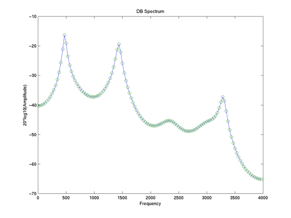
and the (log) amplitude spectrum of this impulse response:
>> lspecplot(fft(impresp),8000);
Now let's figure out what the pole frequencies and amplitudes are:
>> angle(roots(fcoef))*4000/pi
ans =
   1.0e+03 *
    3.2923
   -3.2923
    2.9825
   -2.9825
    2.3412
   -2.3412
    1.4361
   -1.4361
    1.4294
   -1.4294
    0.4731
   -0.4731
    0.6518
   -0.6518
>> abs(roots(fcoef))
ans =
    0.9653
    0.9653
    0.8436
    0.8436
    0.8628
    0.8628
    0.9703
    0.9703
    0.8048
    0.8048
    0.9803
    0.9803
    0.7576
    0.7576
In tabular form, the seven complex poles, corresponding to the seven complex-conjugate roots of the predictor polynomial, have frequencies and amplitudes of
| Frequency in Hz. | Amplitude (0-1) |
|
473.1
|
.9803
|
|
651.8
|
.7576
|
|
1,429.4
|
.8048
|
|
1,436.1
|
.9703
|
|
2,341.2
|
.8628
|
|
2,982.5
|
.8436
|
|
3,292.3
|
.9653
|
Note that by performing a 14-th order analysis, we've guaranteed that we will get seven complex poles (well, we might have substituted a couple of real poles for one of them). If we want to use this method to find the vowel formants, we have to decide which poles correspond to formats and which do not. Here, it is clear (because of the amplitude) that F1 is 473 Hz., and F2 is 1,436 Hz. (though of course the apparent estimation accuracy is spurious). It is less clear what F3 should be.
Suppose we have a causal LTI system S1, with impulse response h, whose z transform, H(z), is a ratio of polynomials B_poly/A_poly.
Now suppose we have another causal LTI system S2, with impulse response g, whose z transform, G(z), happens to be exactly the inverse, namely A_poly/B_poly.
If we convolve some input x with h, and then convolve the result with g -- x # h # g -- this is equivalent to convolving x with the convolution of h with g -- x # ( h # g ).
By the convolution rule for the z-transform, the z-transform of ( h # g ) will be the product H(z)G(z). Given the way we constructed the two systems, this product will be 1 for all values. Therefore the combined system (h # g) will do nothing to its input.
More interestingly, if we already have the output S1(x) = x # h, we can apply the second system to the result to get the original input back: S2(S1(x)) = x. This process is called inverse filtering.
Let's try this with a simple one-pole recursive filter with a center frequency half the sampling rate, excited by an impulse:
r = .95*exp(i*.5*pi);
A= poly([r r']);
impulse=zeros(256,1); impulse(15)=1;
out1 = filter([1 0 0],A,impulse);
 out1(1:30)'
ans =
  Columns 1 through 7
         0         0         0         0         0         0         0
  Columns 8 through 14
         0         0         0         0         0         0         0
  Columns 15 through 21
    1.0000    0.0000   -0.9025   -0.0000    0.8145    0.0000   -0.7351
  Columns 22 through 28
   -0.0000    0.6634    0.0000   -0.5987   -0.0000    0.5404    0.0000
  Columns 29 through 30
   -0.4877   -0.0000
out2 = filter(A,[1 0 0],out1);
out2(1:30)'
ans =
  Columns 1 through 12
     0     0     0     0     0     0     0     0     0     0     0     0
  Columns 13 through 24
     0     0     1     0     0     0     0     0     0     0     0     0
  Columns 25 through 30
     0     0     0     0     0     0
Success! we got the impulse back
Now let's try the recusive filter estimated by the LPC modeling in the previous section. Here we have seven poles -- because we used a 14th-order model. If we apply this filter to a known input -- say an impulse -- and then inverse filter, we'll get our known input back:
[TK]
But it's more interesting to inverse filter the original speech. here we don't actually know what the excitation was, since we are starting from a real-world signal. In fact, the input wasn't really generated by this type of filter at all, but rather by a physical process that is something like -- can be usefully modeled as -- such a filter. So the result of inverse filtering in this case will be a hypothetical signal -- what the input would have been if the output really were created by our modeled filter.
[TK]