Windowing

Let's make 512 samples from 0 to 2*pi*511/512, and sine waves at frequencies 25 and 50:

x = (0:511)*2*pi/512;
y = sin(25*x) + sin(50*x);

Plotting it:

Get the fft and look at the first 60 amplitude values in the frequency domain:

Fy = fft(y); round(abs(Fy(1:60))

ans = Columns 1 through 16: 0 0 0 0 0 0 0 0 0 0 0 0 0 0 0 0 Columns 17 through 32: 0 0 0 0 0 0 0 0 0 256 0 0 0 0 0 0 Columns 33 through 48: 0 0 0 0 0 0 0 0 0 0 0 0 0 0 0 0 Columns 49 through 60: 0 0 256 0 0 0 0 0 0 0 0 0

As we expect, only index values 26 and 51 are non-zero (corresponding to frequencies 25 and 50 because the sequence starts with frequency 0).

We can plot the power spectrum (in the lower-frequency region) on a dB scale (20*log10 of the amplitude spectrum):

aFy = 20*log10(abs(Fy(1:70)));
aFy = aFy-max(aFy);

And we see roughly 250 dB difference between the components we created and the noise floor:

(If you wonder why we use 20*log10 to get the power spectrum values: log10 would give us bels; 10*log10 makes it decibels; and there's an extra factor of 2 because power is amplitude squared...)

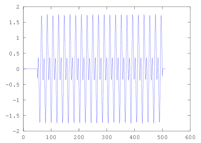
But suppose our analysis window doesn't include an integer number of periods of the frequency-25 and frequency-50 sine waves:

y1 = zeros(512,1);
y1(51:500) = y(51:500);

Now the amplitude spectrum looks quite different:

round(abs(Fy1(1:60)))
ans =
 Columns 1 through 16:
     0     2     3     4     4     4     4     2     1     1     3     5     6     6     6     4
 Columns 17 through 32:
     2     1     5    10    14    19    23    27    29   225    31    29    27    23    18    13
 Columns 33 through 48:
     7     2     3     7    10    12    12    10     7     3     2     7    13    18    23    27
 Columns 49 through 60:
    30    31   225    29    27    23    18    14     9     5     1     2

And the power spectrum shows a radically less crisp separation between the frequencies we put in and the spectrum that we get from the DFT:

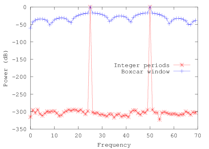
Now the background is less than 18 dB down relative to the peak values -- we've created a lot of spurious structure by violating the DFT's assumption of time-domain periodicity.

Another way to think about what's happened is that we've done an element-wise multiplication, in the time domain, between the original signal and a rectangular window that has the value 1 within the region we're looking at, and 0 outside that region. And just as convolution in the time domain turns into element-wise multiplication in the frequency domain, so element-wise multiplication in the time domain turns into convolution in the frequency domain.

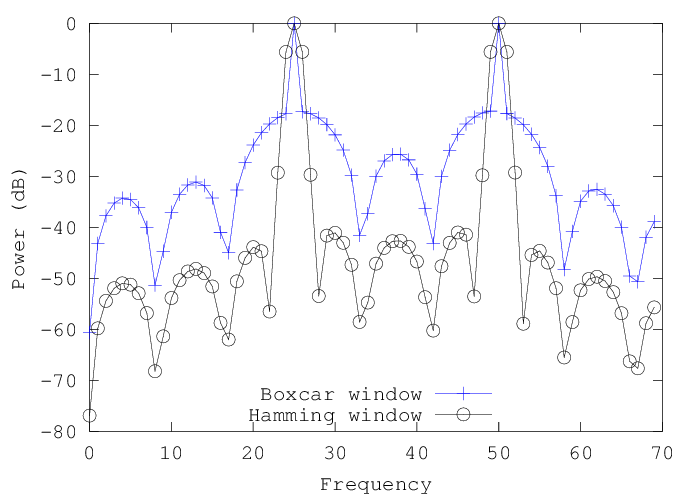
So by using the rectangular (or "boxcar") window on the signal in the time domain, we've convolved the signal's spectrum with the DFT of the window -- and convolving with the DFT of a rectangular window smears out the spectrum in a fairly unpleasant way:

x = zeros(512,1);
x(51:500)=1;
Fx = fft(x);
figure(1)
FFx = abs(fftshift(Fx))(186:325);
plot(-70:69,20*log10(FFx),'r*-')

Any "windowing" -- i.e. selection of regions of a signal for DFT analysis -- will have some effect of this type, but we can choose a window that is better behaved than the boxcar window is. All of the commonly-used windows are symmetrically tapered from a central point to the edges -- usually in some type of bell-shaped curve, starting with the raised inverted cosine called the "hamming window", named after its inventor Dick Hamming:

H = hamming(450);
y2 = zeros(512,1);
y2(51:500) = y(51:500)'.*H;

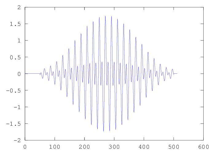
This produces a substantially better difference between the genuine peaks and the splatter created by convolving with the DFT of the window:

And there are some others -- Wikipedia has the details -- that are even better in terms of side-lobe levels, though the main lobe tends to be a bit wider:

But this is not the whole story. Especially when we're dealing with non-stationary signals, we need to think about how to control frequency and time resolution.

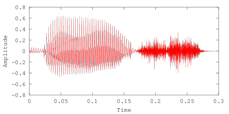
Here's one of the TIMIT calibration sentences:

The waveform shows the syllables unfolding in time:

If we zero in on a single syllable, we can see the periodicity corresponding to the pitch of the voice:

Zeroing in a bit further:

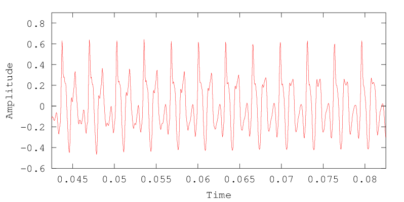
The pitch period in this region is about 3.3 milliseconds, corresponding to a fundamental frequency of a bit more than 300 Hz. If we want to see the pitch in the frequency domain, we'll need an analysis window that includes at least a couple of periods -- otherwise the fact that the periodicity exists will not be available to the analysis.

And if we're using a Hamming window or something similar, we need a bit extra because the edges of the window are attenuated. On the other hand, we don't want too wide a window, because the signal may be changing fairly rapidly. So we might decide to use a window width of 10 msec.

But now we may have another problem. At a sampling frequency of 16000 Hz, 10 msec. is only 160 samples. A 160-element fft will give us 80 samples over the frequency range of 0-8000 Hz., or a frequency resolution of 100 Hz. At this very coarse sampling, we won't see a very clear difference between (say) 300 Hz and 330 Hz, although that difference will be very easy to hear. Changing the sampling rate doesn't help: At an 8000-Hz sampling rate, 10 msec is 80 samples, we so we get 40 samples over 4000 Hz.; at a 48000-Hz sampling rate, 10 msec is 4800 samples, which gives us 2400 samples of range of 24000 Hz. Any way you sample it, 10 msec of digital audio seems to give us only a 100-Hz frequency resolution.

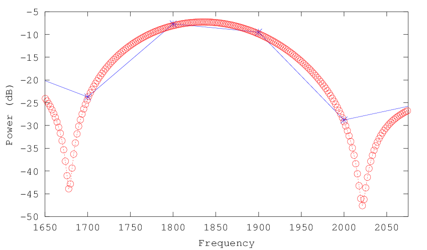
The solution is to embed our 10 msec windowed signal in a longer vector of zeros. This gives us additional frequency resolution without losing time resolution. The plot below shows the frequency range from 0 to 4000 Hz for a 10-msec sample at an 8000 Hz sampling rate. The blue circles show what we get from an 80-sample FFT -- the red line is what we get by embedding the same 80 samples in a 4096-long vector that is otherwise zero, and performing the FFT on that longer input:

And zooming in on one ovetone: