A Bit More on the z-transform and the LPC Spectrum
We start with a linear constant-coefficient difference equation, relating a linear combination of output values to a linear combination of input values:
| Eq. 1 | $$\;\;\;\;\;a_1 y[n] + a_2 y[n-1] + ... + a_{M+1} y[n-M] = b_1 x[n] + b_2x[n-1] + ... + b_{N+1} x[n-N]$$ |
(The input is x and the output is y, and here we've started indexing the coefficients from 1 upwards, rather than from 0 upwards, to accord with the usage in Octave's filter() function.)
Or equivalently
| Eq. 2 | $$\sum_{k=0}^N a_{k+1} y[n-k] = \sum_{k-0}^M b_{k+1} x[n-k] \;\;\;\;\;\;for \;\;1 <=n<=length(x)$$ |
A little algebra gives us a form of the equation expressing the current output y[n] as a linear combination of inputs and outputs:
| Eq. 2 | $$y[n] = -\sum_{k=1}^N c_{k+1} y[n-k] + \sum_{k=0}^M d_{k+1} x[n-k] \;\;\;\;\;\;for \;\;1 <=n<=length(x)$$ |
where \(c = a/a_1 \;\; and \;\; d = b/a_1\).
Notice that for an Nth-order autoregressive model -- predicting each output as a linear combination of N previous samples -- there are N+1 \(a\) coefficients, as in equations 1 and 2 above, with the first coefficient by convention equal to 1. And for an "all-pole" filter -- a purely autoregressive model, with no moving-average part -- we still need a dummy \(b\) vector, with 1 as the first coefficient (thereby passing in the current input sample, to be combined with the weighted combination of earlier outputs.
The Octave/Matlab function filter() is invoked as
y = filter (b, a, x);
where x is the input vector, b and a are the input and output coefficients as in equations 1 and 2, and y is the output vector.
In the lecture notes, you learned how to calculate a as the solution to a problem in linear regression. Here we'll just use the arburg() function from the signal package, which we can invoke as
a = arburg(x, npoles);
Let's analyze this sentence from the TIMIT corpus:
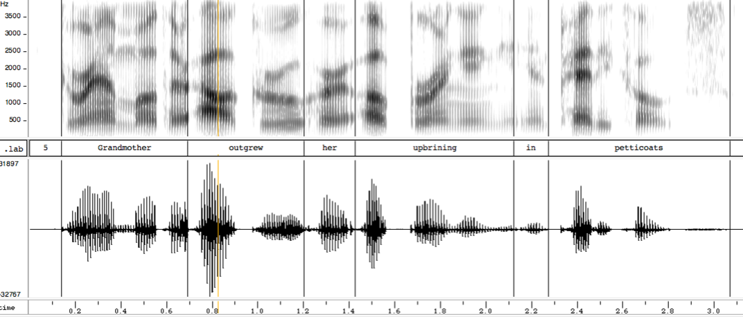
The vertical line in the first syllable of "outgrew" is at about 0.823 seconds. So we do this:
[X, FS] = wavread("SX48a.wav");
windowT = 0.03;
windowN = round(windowT*FS);
T1 =  0.823;
T1n = round((T1-windowT/2)*FS);
S1 = X(T1n:(T1n+windowN-1));
NOrder = 10;
A1 = arburg(S1,NOrder);
This gives us 11 a coefficients calculated for the cited region of the audio clip:
A1 =
   1 -1.4778 1.0066 -0.17666 0.33168 0.029883 -0.21203 -0.19413 0.91318 -0.63106 0.18872
We can ask Octave for the (complex) roots of the polynomial, of which there are 5 complex-conjugate pairs:
roots(A1)
ans =
    -0.82266 +    0.37935i
    -0.82266 -    0.37935i
    -0.28849 +    0.92907i
    -0.28849 -    0.92907i
     0.61941 +    0.72331i
     0.61941 -    0.72331i
      0.8242 +    0.49916i
      0.8242 -    0.49916i
     0.40646 +    0.35125i
     0.40646 -    0.35125i
Or more helpfully, we can get the 5 frequency and amplitudes (translating the frequencies from radians into Hz):
R1 = roots(A1)(1:2:9);
Freqs = angle(R1)*(FS/2)/(2*pi);
Amps = abs(R1);
[Freqs Amps]
ans =
    1724.9     0.90591
    1191.7     0.97282
    549.17     0.95229
    346.67     0.96357
    453.7      0.5372
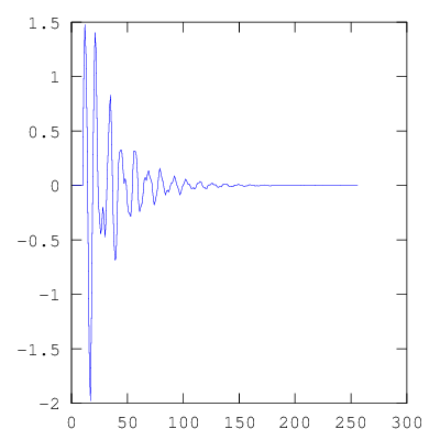
We can calculate and plot the impulse response:
NFFT=256;
Impulse = zeros(NFFT,1); Impulse(NOrder+1)=1;
ImpulseResponse = filter([1 0],A1,Impulse);
plot(1:NFFT,ImpulseResponse)
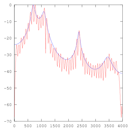
And we can compare the power spectrum of the impulse response with the power spectrum of the original signal:
NFFT=512; NFFT2 = NFFT/2;
freqs = (0:(NFFT2-1))*(FS/2)/NFFT2;
% Power Spectrum of LPC Impulse Response:
IR1 = zeros(NFFT,1); IR1(1:length(ImpulseResponse)) = ImpulseResponse;
psd1 = 20*log10(abs(fft(IR1)(1:NFFT2)));  psd1 = psd1-max(psd1);
% Power Spectrum of input signal (with Hamming window):
S1a = hamming(length(S1)).*S1;
xx = zeros(NFFT,1); xx(1:length(S1a)) = S1a;
psd2 = 20*log10(abs(fft(xx)(1:NFFT2)));  psd2 = psd2-max(psd2);
% Plot both:
plot(freqs, psd1,'b',freqs,psd2,'r')
As we discussed in the lecture notes on the z-transform, we can also estimate the spectrum of the autoregressive filter directly from the z-transform of \(H(z)\), which in the case of a purely autoregressive filter is
$$\frac{Y(z)}{X(z)} = \frac{1}{ 1 + a_1 z^{(-1)} + ... + a_M z^{(-M)} }$$
Since we know that the z-transform reduces to the DTFT for \(z=e^{iw}\), and we know how to calculate the z-transform of any causal LTI (i.e. the z-transform of its impulse response) from the coefficients of the difference equation, we can write down an expression for the spectrum of the filter (i.e. the ratio of the spectrum of the output to the spectrum of the input) by simply setting \(z=e^{iw}\) in the z-transform.
This expression will be a periodic, continuous function of the variable w, which is frequency in radians. The period is obviously \(2pi\). We can get N evenly-spaced samples of one period of the spectrum (which is also what the DFT gives us) by setting (in Matlab-ish) w = ((0:(N-1))/N)*2*pi, i.e.
$$z=e^{i(n/N)2\pi}\;\;\;\;for\;0<=n<=N-1$$
Of course, given that we only want the positive frequencies, we should limit the evaluation to w = ((0:(N-1)/N)*pi.
So let's do it:
N=256;
w = ((0:(N-1))/N)*pi;
Hz = zeros(N,1);
for n=1:N
    z = exp(i*w(n));
    Hz(n) = 1/(A1*z.^(-(0:NOrder))');
end
psd3 = 20*log10(abs(Hz)); psd3 = psd3-max(psd3);
plot(freqs,psd3,'mo',freqs,psd1,'b')
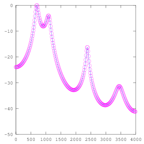
We see that the two ways of calculating the LDC spectrum -- by taking the FFT of the impulse response of the filter, and by evaluating the z-transform at suitable points around the unit circle -- produce identical results. You should be able to figure out for yourself how to evaluate the z-transform in its factored form.