Goals:

• Getting Octave (or Matlab) set up on your computer
• Doing arithmetic on scalars, vectors and matrices;
  for loops;
  simple use of plot( ) and imagesc( ) .
• Loading audio data using wavread().
• Running a file of commands as a script (a .m file).

Your answers should be in the form of an executable m-file, named "YourNameHW1.m" -- thus if your name were Kim Lee, your m-file would be named "KimLeeHW1.m". Please check that your file can actually be executed before submitting it. Upload your solution to the course canvas site (which should be created in time for the submission...). If you want to add any commentary, use the comment character % to do so.

This set of directions does not include an adequate tutorial introduction to Octave, though if you are familiar with similar computer languages, you may be able to get by. Many tutorials are available on line, e.g here or here, or you can attend an introductory lab session which we will schedule if there is enough interest.

In order to read data from an external file, it must be in a folder or directory that Octave or Matlab can "see". The way(s) to do this vary somewhat with the program, the release, and the operating system. This may involve placing the file in a special directory; and/or invoking Octave or Matlab in the directory in question; and/or using the path( ) command; and/or ... Note that from inside Octave you can get some useful information by invoking e.g.

>> help("path")

If you run into any persistent trouble with this or any other issue, please ask for help.

The file SX133.wav. contains an audio file from the TIMIT dataset -- the text is "Pizzerias are convenient for a quick lunch". Download this file from the link just given, and read it into Octave using the command

>> [X, FS] = wavread("SX133.wav");

[In MATLAB, the corresponding function is audioread().]

Now the value of FS is the file's sampling frequency, which in this case is 16000 samples per second:

>> FS
FS = 16000

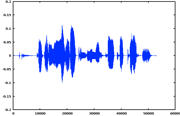
and X is a vector of 53,044 numbers representing sequential samples of the speech waveform:

>> plot (X)

[In MATLAB, and in some recent versions of Octave, you can play an audio file with a command like

>> soundsc(X,FS);

If this doesn't work in your environment, you can use a free waveform editor like Audacity to display and play the file (outside of Octave).]

At this point, you'll want to start putting your code into a script that you can modify, revise, execute, and eventually submit. In order to create a script that you can run in Octave, create a text file whose name ends in ".m" (like "foo.m" or "KimLeeHW1.m" or whatever), in an accessible directory or folder. Then you should be able to type

>> foo

in Octave and have the contents of the file executed as if you had typed them. (Note that such scripts need to be plain text files, not e.g. Microsoft Word files...)

What follows is some background discussion, and then (at last!) your two-part assignment.

Background

If (after reading in the audio file) you execute a script containing

s1 = round(0.98*FS); s2 = round(1.11*FS);
plot((s1:s2)/FS, X(s1:s2))

you'll see this plot of (roughly) the /ri/ syllable of "pizzeria":

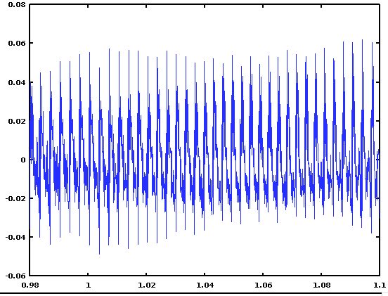
Make sure you understand what those two lines of code are doing.

In the plot, you can see the quasi-periodic oscillations that correspond to the fundamental frequency (or F0) of the speaker's voice in that region. There are many ways to estimate the periodicity in data of this kind, but one common method is to look at the "serial cross-correlation" of the signal with itself.

Let's see how this works, by taking 10 msec of data (160 samples at 16000 Hz sampling rate), starting 1 second into the utterance, and calculating its correlation with 10-msec pieces starting up to 20 msec (320 samples) later, increasing the lag from 1 to 320 samples, one sample at a time. The idea is that this serial cross-correlation is a good measure of the similarity of the signal to itself at a given lag; and that self-similarity, in turn, is what "(quasi-)periodicity" really means. Here's what the Octave code might look like:

[X, FS] = wavread("SX133.wav");
s1 = round(0.98*FS); s2 = round(1.11*FS);
figure(1)
plot((s1:s2)/FS, X(s1:s2))
%
start = round(1.0*FS);
nwindow = round(0.01*FS);
nlags = round(0.02*FS);
SCC = zeros(nlags,1);
base = X(start:(start+nwindow-1));
for n=1:nlags
SCC(n) = corr(base, X((start+n):(start+n+nwindow-1)));
end
figure(2)
plot((1:nlags)/FS, SCC)

The resulting serial cross-correlation plot will look like this:

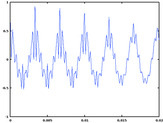
The sequence of peaks represents lags of one, two, three, four, five, etc., periods in the signal.

In this case, the highest peak is at a lag of 53 samples:

>> [val, ind] = max(SCC)
val = 0.92636
ind = 53

which corresponds to a period of 53/16000 = 3.3125 msec., or a frequency of 16000/53 = 301.89 Hz.

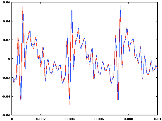
A plot shows us that the two signal subsequences really really are quite similar at the lag corresponding to the correlation peak:

>> plot((1:nwindow)/FS, X(start:(start+nwindow-1)), 'r', (1:nwindow)/FS, X((start+53):(start+53+nwindow-1)), 'b')

If we wanted a more accurate estimate, we would use quadratic interpolation to find the period more exactly, by more accurately estimating the peak location as a fractional lag given the values at lags 52:54 -

>> SCC(52:54)
ans =
0.39725
0.92636
0.84806

If we temporarily assign the x coordinates [-1 0 1] to three y values [a b c], a bit of high-school algebra tells us that the peak location can be calculated as

x = (1/2)*(a-c)/(a-2*b+c)

Or in this case,

>> y=SCC(52:54);
>> xloc = (1/2)*(y(1)-y(3))/(y(1)-2*y(2)+y(3));
>> BestLag = 53+xloc;
>> Period = BestLag/FS; F0 = FS/BestLag;

which produces an interpolated lag estimate of 53.371, a new estimated period of 3.3357 msec., and a new estimated F0 of 299.79.

Assignment 1

Write a script to apply the serial cross-correlation calculation 100 times per second (i.e. re-starting every ten milliseconds) to the file we've been working with. The usual terminology is to call the results of each such calculation a "frame". How many frames will there be?

In this case, the increment is an integer number of frames (.01*16000 = 160), but let's use a method that would also work if the sampling rate were e.g. 11025, where the increment would not be an integer (.01*11025 = 110.25).

We need to start the last SCC calculation with room for nlags delayed copies of nwindow, and the nth frame starts at sample number round((n-1)*increment*FS) -- the "-1" is because Octave's array numbering starts from 1 rather than from 0. So we need (nframes-1)*increment*FS < nsamples-(nlags+nwindow). And therefore in Octave:

nframes = floor( (nsamples-(nlags+nwindow+1))/(increment*FS) ) + 1;

which works out to 329 for the cited file. The result should thus be a matrix whose columns correspond to the 329 analysis frames, and whose rows correspond to the 320 lags. The value in cell i,j should then be the cross-correlation for the jth starting time and the ith lag. You might set this up as e.g.

>> Correlogram = zeros(nlags,nframes);

Then after filling the matrix with appropriate values, you should plot it as a "correlogram" using imagesc(). Since the use of this function is a bit opaque, here's a recipe for doing the right thing:

% lag values in msec:
yvalues = ((1:nlags)/FS)*1000;
% time values in seconds:
xvalues = (0:(nframes-1))*increment;
imagesc(xvalues, yvalues, correlogram);
% force imagesc() to plot first row at the bottom of the image
set(gca,'YDIR', 'normal');

Assignment 2

Now, based on the correlogram matrix produced in the previous step, calculate the F0 corresponding to the best-scoring lag at each cross-correlation frame.

You probably will have noticed that the correlogram calculation takes several minutes -- Octave for-loops are rather slow -- so you will probably want to save the correlogram from step 1 -- a good way to do this is

save corr.mat correlogram

which will save the variable "correlogram" in binary form to a file named "corr.mat". You can read this in later on using

load corr.mat

We can decide a priori that the pitch must be between (say) 50 and 500 Hz -- these correspond to lags (in samples) of

>> round(FS/500)
ans = 32
>> round(FS/50)
ans = 320

If you look at the documentation for the max() function -- via e.g. help("max") -- you'll see that you can get the maximum values and indices within those bounds using a sequence like

[vals, inds] = max(correlogram(32:320,:));
inds = inds+31;

The pitches corresponding to these lags are then just

F0 = FS./inds;

When you plot these, you'll see that there are a lot of ridiculous points in the regions where the signal is silent or noisy rather than quasi-periodic. So you'll want to plot using isolated points rather than (the default) connected lines, e.g. a FMT of something like '.ro', which will plot red o's at the given points, e.g.

times = ((1:nframes)-0.5)*increment;
plot(times, F0, '.ro')

Unfortunately, the function plotyy() -- which lets us compare two sequences on the same plot with different y-axis scaling -- doesn't seem to allow plotting points rather than lines. So as second best, we can put two plots above one another:

subplot(2,1,1)
plot(times, F0, '.ro')
subplot(2,1,2)
plot(times,vals,'-b')

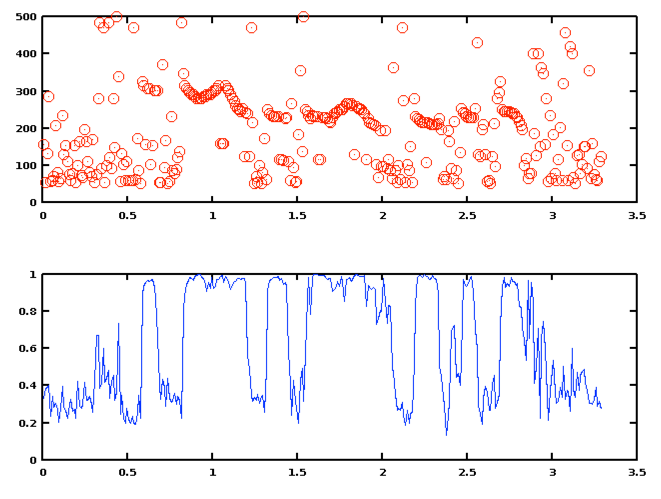
You can now see how modern pitch trackers use a combination of voicing determination and continuity constraints to clean up the answers that they give -- and perhaps you can also begin to see why complete clean-up is usually not possible, even for relative clean recordings of single voices without pathologies.

To complete this assignment, adjust the period estimates (and therefore the F0 estimates) using quadratic interpolation as explained above. (Note that given the restriction of the max() function to a limited range of lags, not all registered locations will actually be local maxima -- you need to check that the index of maximum is not the first or last of the allowable indices, before doing the interpolation...)