First steps with R
In this lesson, you'll do three things:
1. Download a small dataset.
2. Learn by example to read this dataset into R and do some simple things with it.
3. Download a short R script that does some other simple things with this dataset, and modify that script to do a couple of equally simple but slightly different things.
The modified script is what you'll hand in.
Optionally, you can work through the first few sections of one of the many online R tutorials, for example this one.
1. The NHANES1 Dataset
The National Health and Nutrition Examination Survey (NHANES)
is a program of studies designed to assess the health and nutritional status of adults and children in the United States. The survey is unique in that it combines interviews and physical examinations. NHANES is a major program of the National Center for Health Statistics (NCHS). NCHS is part of the Centers for Disease Control and Prevention (CDC) and has the responsibility for producing vital and health statistics for the Nation.
Out of the many datasets available for the 2009-2010 NHANES cycle, I've selected a few variables from the Demographics Data and a few variables from the Examination Data. NHANES calls these
SEQN "Respondent sequence number"
RIAGENDR "Gender of the sample person"
RIDAGEEX "Best age in months at date of examination for individuals under 80 years of age at the time of MEC Exam"
RIDRETH1 "Recode of reported race and ethnicity information"
BMXWT "Weight (kg)"
BMXHT "Standing Height (cm)"
BMXWAIST "Waist circumference (cm)"
I've pulled these out of the original SAS .xpt files and combined them into a text file under the names
ID SEX AGE ETH WT HT WAIST
That file can be found at http://ling.upenn.edu/courses/ling005/NHANES1.txt.
Using cntl-click>>Save Link As (Mac OSX) or right-click>>Save link as... (Windows), save this file in whatever folder you plan to use for your work in this course.
2. Some simple interactions in R with this dataset
Then in R, make sure that the "working directory" is set to that location.
In any R implementation, you can do this with the command
setwd("PathToFolder")
Or you can do it interactively via Misc>>Change Working Directory... (Mac OSX) or File>>Change dir... (Windows).
Now you should be able to read in the NHANES1.txt dataset in the R console, like this:
X = read.table("NHANES1.txt")
The R variable X now refers to a dataframe whose dimensions we can find out this way:
> dim(X)
[1] 10253     7
(Here the '>' character is the R console prompt, and the line beginning with [1] is the two-element vector that tells us the number of rows (10253) and columns (7) in X.)
We can reference the ith row and jth column of X via the expression
X[i,j]
If we leave out i or j, the reference defaults to the whole row or column. Thus
> X[1,]
      ID SEX AGE ETH   WT    HT WAIST
 1 51624   1 410   3 87.4 164.7 100.4
 > X[306,]
        ID SEX AGE ETH   WT  HT WAIST
 306 51937   1 139   1 28.3 142  57.6
shows us the first and the 306th rows of X. And because e.g.
> 11:20
[1] 11 12 13 14 15 16 17 18 19 20
we can see rows 11 through 20 of X this way:
> X[11:20,]
      ID SEX AGE  ETH    WT    HT WAIST
11 51634   1 121    1  44.7 143.6  78.9
12 51635   1  NA    3  89.6 180.1 113.7
13 51638   1 116    3  29.8 133.1  60.6
14 51639   1  59    1  17.9 103.0  51.2
15 51640   1 209    2  74.7 169.6  86.0
16 51641   1 156    4  40.6 156.4  63.6
17 51642   1  85    1  22.2 120.2  56.3
18 51643   2 516    4 107.7 164.3 129.8
19 51644   1  10    3   9.3    NA    NA
20 51645   1 797    1  82.9 171.3    NA
"NA" means "Not Available" -- those are values that are missing from the table, for whatever reason.
We can also refer to columns by name rather than by number, so that
X[,5]
and
X[,"WT"]
both refer to the fifth column of X, "weight in kilograms".
If we ask for the average value of the weight column, we get an unpleasant surprise
> mean(X[,5])
[1] NA
because R isn't sure what we want to do with the NA values, so NA propagates to the result of the calculation.
We can avoid this outcome by using setting the parameter na.rm in the call to mean():
> mean(X[,"WT"], na.rm=TRUE)
[1] 63.29224
The same thing applies to many other functions, for example var() which calculates the variance of a set of numbers. Thus to calculate the standard deviation of the WT values
> sqrt(var(X[,"WT"]))
[1] NA
> sqrt(var(X[,"WT"],na.rm=TRUE))
[1] 32.35685
The function summary(), however, doesn't have to be told:
> summary(X[,"WT"])
   Min. 1st Qu.  Median    Mean 3rd Qu.    Max.    NA's
   2.70   39.20   66.80   63.29   84.40  239.40      91
The column that I've labelled "ETH" is called "RIDRETH1" ("Recode of reported race and ethnicity information") by NHANES, and subdivided as follows:
(1) "Mexican-American"
(2) "Other Hispanic"
(3) "non-Hispanic white"
(4) "non-Hispanic black"
(5) "other race including multiracial"
So the numbers from 1 to 5 in this column are not really numbers, but references to the levels of a kind of variable that R calls a "factor". If we ask R to summarize this column, it will dutifully give us meaningless information about quantiles, as if 1-5 really meant 1-5. So we need to tell R to treat those values appropriately:
> summary(X[,"ETH"])
   Min. 1st Qu.  Median    Mean 3rd Qu.    Max.
   1.00    2.00    3.00    2.75    3.00    5.00
> summary(as.factor(X[,"ETH"]))
   1    2    3    4    5
2305 1103 4317 1903  625
This tells us that there are 2305 rows with factor level 1, 1103 rows with factor level 2, etc.
Some operators produce "boolean" (TRUE or FALSE) results. This applies to relational operators on numerical values, like
> 7:15
[1]  7  8  9 10 11 12 13 14 15
> (7:15) > 9
[1] FALSE FALSE FALSE  TRUE  TRUE  TRUE  TRUE  TRUE  TRUE
We can also use it to select certain levels of a factor. Thus to select "Mexican-American" people in the NHANES dataset:
> X[1:20,"ETH"]
 [1] 3 5 4 4 4 1 3 3 2 3 1 3 3 1 2 4 1 4 3 1
> X[1:20,"ETH"]==1
 [1] FALSE FALSE FALSE FALSE FALSE  TRUE FALSE FALSE FALSE FALSE  TRUE FALSE FALSE
[14]  TRUE FALSE FALSE  TRUE FALSE FALSE  TRUE
We can assign such a boolean vector to a variable:
> MexicanAmerican = (X[,"ETH"]==1)
One useful thing to do with a Boolean vector is to count its TRUE values, e.g.
> sum(MexicanAmerican)
[1] 2305
More important, we can use such a vector as a subscript for a vector or matrix or dataframe. Thus X[MexicanAmerican,] gives us the rows corresponding to Mexican-American sample persons, and
> mean(X[MexicanAmerican,"HT"],na.rm=TRUE)
[1] 150.1403
gives us the average weight of people in that category.
We can also combine boolean vectors with operators like '&' ("and"), '|' ("or"), etc. So
> female = (X[,"SEX"]==2)
> male = (X[,"SEX"]==1)
> adult = (X[,"AGE"] >= 18)
> h1 = mean(X[MexicanAmerican & adult & female,"HT"], na.rm=TRUE)
> h2 = mean(X[MexicanAmerican & adult & male,"HT"], na.rm=TRUE)
And thus
> h1   # average height of Mexican-American adult females in the sample
[1] 146.0263  # cm
> h2   # average height of Mexican-American adult males in the sample
[1] 153.9839  # cm
> h2/h1 # Ratio
[1] 1.054494   # males are 5.4% taller
3. Running, understanding, modifying script1.R
You should now be able to follow what's going on in script1.R -- download it to your working directory, and execute it in the R console window via
> source("script1.R")
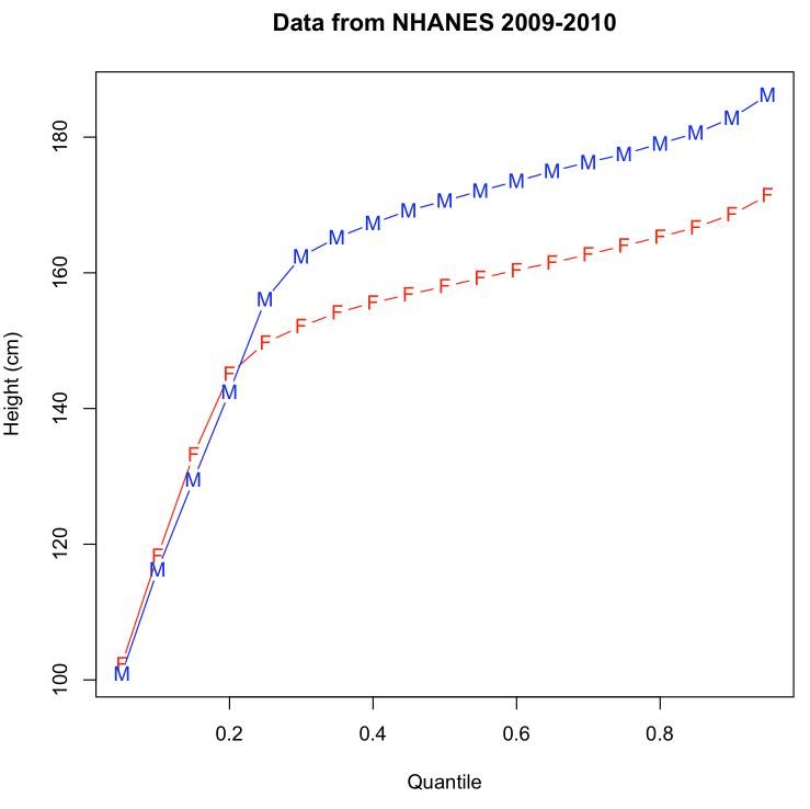
It should produce a plot that looks more or less like this:
Note that if there are things in the script that puzzle you, you can get help within the R console by e.g.
> help(plot)
If that doesn't give you the information you need, try asking a question on the Piazza site.
Your assignment is to do two simple things:
(1) It may seem puzzling at first that female height runs slightly ahead of male height up to about the 25th percentile. But there's a simple reason -- can you guess why this might be true? What small change to the script would support your hypothesis? (Express your answer via comments -- lines starting with '#' -- in a modified R script.)
(2) Further modify the script to make analogous plots for weight and waist circumference. Note that if you want to put all the plotting instructions in one R script file, it will help to insert the command
> par(ask=TRUE)
which will tell R to ask you before replacing each plot with the next one.
How should you modify the script? You could use a plain text editor outside of R, e.g. TextEdit (on Mac OSX) or Notepad (on Windows) -- though you'll have to be sure that the editor is really saving your file as plain text, without spurious formatting instructions. A (probably) more reliable alternative is to use the editor built into the R GUI, reading the script in via File>>Open Document (OS X) or File>>Open Script... (Windows), and writing out your modified version via File>>Save As...