Statistical estimation for Large Numbers of Rare Events
It often happens that scientists, engineers and other biological organisms need to predict the relative probability of a large number of alternatives that don't individually occur very often. This is especially troublesome in cases where many of the things that happen have never happened before: where "rare events are common".
The simple "maximum likelihood" method for predicting the future from the past is to estimate the probability of an event-type that has occurred r times in N trials as r/N. This generally works well if r is fairly large (and if the world doesn't change too much). But as r gets smaller, the maximum likelihood estimate gets worse. And if r is zero, it may still be quite unwise to bet that the event-type in question will never occur in the future. Even more important, the fraction of future events whose past counts are zero may be substantial.
There are two problems here. One is that the r/N formula divides up all of the probability mass -- all of our belief about the future -- among the event-types that we happen to have seen. This doesn't leave anything for the unseen event-types (if there are any). How can we decide how much of our belief to reserve for the unknown? And how should we divide up this "belief tax" among the event-types that we've already seen?
The second problem looks even harder. Suppose we think we know how much probability to hold back for unseen events -- does this mean that all unseen event-types get an equal share? In many practical cases, our intuition tells us that this is not true. Thus as of this moment, Google's index happens not to include the character sequence "eleven gaslights". But we can be pretty confident that its probability of occurrence in the future is greater than the probability of some random permutation of the same letters, e.g. "tieegvl asnlhsge".
This is closely related to the problem of getting better estimates for the future chances of event-types that we've seen a small number of times. There is often some structure in the event space that allows us to use other sorts of evidence to improve such predictions -- for example, by relating the probability of symbol-sequences to the probabilities of sub-sequences involving the same symbols.
For solving the first problem, a key paper is IJ Good, "The Population Frequencies of Species and the Estimation of Population Parameters", Biometrika 40(3-4) 237-264, December 1953. The abstract:
A random sample is drawn from a population of animals of various species. (The theory may also be applied to studies of literary vocabulary, for example.) If a particular species is represented r times in the sample of size N, then r/N is not a good estimate of the population frequency, p, when r is small. Methods are given for estimating p, assuming virtually nothing about the underlying population. The estimates are expressed in terms of smoothed values of the numbers nr (r = 1, 2, 3, ...), where nr is the number of distinct species that are each represented r times in the sample. (nr may be described as `the frequency of the frequency r'.) Turing is acknowledged for the most interesting formula in this part of the work. An estimate of the proportion of the population represented by the species occurring in the sample is an immediate corollary. Estimates are made of measures of heterogeneity of the population, including Yule's 'characteristic' and Shannon's 'entropy'. Methods are then discussed that do depend on assumptions about the underlying population. It is here that most work has been done by other writers. It is pointed out that a hypothesis can give a good fit to the numbers nr but can give quite the wrong value for Yule's characteristic. An example of this is Fisher's fit to some data of Williams's on Macrolepidoptera.
One of the most straightforward results of this interesting paper is that (where N is the total observed count of individuals),
the expected total chance of all species that are each represented r times ... in the sample is approximately
(r+1)nr+1/N
and as a result,
We may say that the proportion of the population represented by the [species in the] sample is approximately 1−n1/N, and the chance that the next animal sampled will belong to a new species is approximately
n1/N
This gives us a simple and elegant answer to the question of how much of our belief we should reserve for things we haven't seen yet.
And as Good explains, this result is based on only very weak assumptions about the population distribution and the sampling process: we assume only that the distribution remains constant as samples are taken, and that each individual sampling event is independent of the others.
(It's worth observing that even this rather weak assumption may be false in real situations, in particular where the "animals" being sampled run in herds or flocks or swarms.)
Let's check this out in a few concrete cases.
First, a simple artificial case.
Let's generate (in Matlab) 100 integers between 1 and 1000, from a uniform distribution:
nums = 1:1000;
X = round(random('unif',1,1000,100,1)); % 100 random ints
types = length(unique(X)); % number of types
counts = histc(X,nums); % histogram of values
N1 = sum(counts==1); % number of singletons
If we do this five times, we get type counts in our samples of types = 93, 98, 96, 92, 95.
And we get singleton counts of n1 = 86, 96, 92, 84, 90.
The Good-Turing estimate of the proportion of the population represented by our sample is supposed to be "approximately 1−n1/N", which in this case is
>> 1-N1./100
ans =
0.1400 0.0400 0.0800 0.1600 0.1000
In this case, since the distribution is uniform by construction, we can turn these proportions into estimated counts of unseen types:
>> round(types./(1-N1./100))
ans =
664 2450 1200 575 950
which is not terrific, but not totally nuts either. The mean of those five estimates is 1,168, which is within 17%.
If we increase the sample size to 500, and take five samples, as before, we get types = 402, 381, 393, 405, 388; N1 = 314, 279, 304, 323, 292; and
>> round(types./(1-N1./500))
ans =
1081 862 1003 1144 933
These individual estimates are much closer, and their average is 1,004.6, which is very close to the truth.
Let's try a different artificial case, using the negative binomial distribution.
In successive random trials, each with a constant probability P of success, the number of trials required in order to observe a given number R of successes has a negative binomial distribution with parameters R and P. Thus if we set R to 1, and P to the probability that the next word in a text is "whatever", then nbinpdf(R,P) gives us the probability distribution over intervals between occurrences of "whatever".
Here's a picture of what this distribution looks like:
>> X=random('nbin', 1, .005, 100000, 1);
>> hist(X,1000)
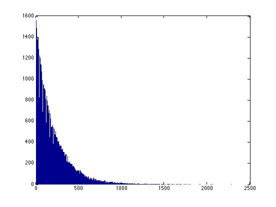
Note that there's no limit to the possible size of these intervals -- for any interval, no matter how large, there's a finite (but perhaps very small) probability that we might have to wait that long to see "whatever". Thus it's not helpful to ask "how many possible intervals are there?" because the answer is "infinitely many".
However, it still might make sense ask (and answer) questions like "what proportion of the population is represented by the types (i.e. the intervals) in our sample?", or equivalently, "how much of our belief should we hold back for so-far-unseen types?". The easiest way to check this will be to see what proportions of new samples belong to unseen types.
We'll take 5 samples of 500 each; from each sample, we'll calculate Turing's estimate of what proportion of the population is covered by the types in our sample, and therefore what the probability of new types in new samples should be; and we'll compare that against what we learn by comparing the five samples to one another.
nums = 1:10000;
Tokens = 500;
types = zeros(5,1); N1 = zeros(5,1); X = zeros(5,Tokens);
for m=1:5
X(m,:) = random('nbin', 1, .005, Tokens, 1);
types(m) = length(unique(X(m,:)));
counts = histc(X(m,:),nums);
N1(m) = sum(counts==1);
end
%
Cnew = zeros(5,5);
for n = 1:5
for m = 1:5
hn = histc(X(n,:),nums); hm = histc(X(m,:),nums);
for v = 1:10000
if(hn(v)==0 && hm(v)>0)
Cnew(n,m) = Cnew(n,m)+hm(v);
end
end
end
end
Cnew = Cnew./Tokens;
Our average prediction for the probability of seeing new types is
mean(N1./Tokens)
which in this case turns out to be 0.3664. The actual proportion of new types (in a sample of 500), averaged across the other five samples, is
(sum(sum(Cnew)) - sum(diag(Cnew)))/20
which in this case comes out to 0.3872. If we increase the sample size to 5,000, the Good-Turing estimate of the probability of seeing new types falls to 0.0393, and the empirical test turns out to be 0.0403.
Let's try this in a real-world example.
In the first 100,000 words of a corpus of conversational speech, there are 5,978 distinct word types, 2,748 of which occur only once.
Thus the Good-Turing estimate of "the chance that the next animal sampled will belong to a new species" is 2,748/100,000, or about 1 in 36.4.
In fact, of the next 100,000 words in the corpus, 2,510 are new, or about 1 in 39.8 -- that's about 9% fewer "new species" than the Good-Turing estimate.
In the first 200,000 words, there are 8,488 distinct word types, of which 3,663 occur just once. This predicts a new-species rate of 3,663/200,000, or about 1,832 per 100,00 (about 1 in 54.6).
In fact, when we look at the third set of 100,000 new words in the corpus, we see 1,943 new words (relative to the first 200,000), or about 1 in 51.5. That's about 6% more "new species" than the Good-Turing estimate.
Iterating again, the first 300,000 word tokens include 10,341 word types, of which 4,282 are singletons. This predicts a new-species rate of 4,282/300,000, or about 1,427 per 100,000 (about 1 in 70.1).
When we try it, we find that the next 100,000 words include 1,572 new word types (relative to the first 300,000), or about 1 in 63.6. That's about 10% more than the Good-Turing estimate.
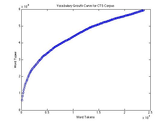
The empirical type/token curve (showing vocabulary growth) for 23.7 million words of conversational speech transcripts looks like this:
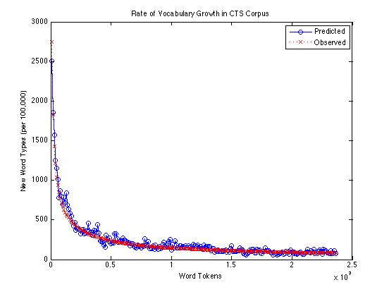
If we compare the Good-Turing estimate of the rate of appearance of new words with the actual count of new words found (per 100,000 tokens), over the same corpus, it looks like this:
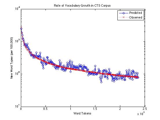
Or on a log scale:
And here's just the difference between observed and predicted counts of new words:
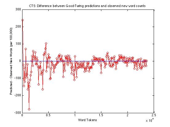
Across the whole range -- from 100,000 to 23,600,000 -- the Good-Turing method is under-predicting the rate of occurrence of new words by an average of about 14.2 words per 100,000. From a million words up, the average underprediction is about 13.6 words per 100,000; from ten million words up, the average is about 7.8.
So the Good-Turing method is doing a decent job of telling us how much of our belief to hold back for previously-unseen words. Now how should we distribute this "belief tax" across the probability estimates for the words that we *have* seen?
Well, the Good-Turing answer is simple in theory. Given a word w that occurs r times out of N total word tokens, where the number of words occurring r times is nr, we should estimate P(w) as r*/N, where
r* = (r+1)*nr+1/nr
This is fairly easy for the rare words. In the CTS corpus just discussed, after 23.7M words, the low-frequency end of this spectrum looks like this:
| 1 | 19,026 |
0.7573 |
| 2 | 7,204 |
1.7619 |
| 3 | 4,231 |
2.7152 |
| 4 | 2,872 |
3.6856 |
| 5 | 2,117 |
4.7246 |
| 6 | 1,667 |
5.9418 |
| 7 | 1,415 |
6.4339 |
| 8 | 1,138 |
8.0193 |
| 9 | 1,014 |
8.0473 |
| 10 | 816 |
Thus we can calculate r* for r=1 as 2*7,204/19,026 = 0.7573; and r* for r=2 as 3*4,231/7,204; etc.
But as we work our way towards the high-frequency end of the spectrum, we'll run into problems. The observed values for nr become noisy, and many of them are 0:
| 1000 | ||
| 1001 | ||
| 1002 | ||
| 1003 | ||
| 1004 | ||
| 1005 | ||
| 1006 | ||
| 1007 | ||
| 1008 | ||
| 1009 | ||
| 1010 |
The thing is, we should really be using the expected values of nr -- the values that we would converge on if we took many samples from the same population. Then the equation for r* becomes
r* = (r+1)*E(nr+1)/E(nr)
At the low-frequency end, where the nr counts are high, the empirically-observed ratio nr+1/nr is generally going to be pretty close to what we want. But as the counts go down, the "maximum likelihood" estimates get worse and worse.
In Good's 1953 paper (cited above) he observes:
The purpose of smoothing the sequence n1, n2, n3, ... and replacing it by the new sequence n'1, n'2, n'3, ..., is to be able to make sensible use of the exact results (14) and (15). ... [T]he best value of n'r would be EN(nr|H) where H is true. One method of smoothing would be to assume that H = H(p1, p2, ..., ps) belongs to some particular set of possible H's, to determine of these, say H0, by maximum likelihood and then to calculate n'r as EN(nr|H0). ... Since one of our aims is to suggest methods which are virtually distribution-free, it would be most satisfactory to carry out the above method using all possible H's as the set form which to determine H0. Unfortunately, this theoretically satisfying method leads to a mathematical problem that I have not solved.
He discusses using free-hand curves, "smoothed two or three times, perhaps by different people"; and he suggests that
... rather than working directly with n1, n2, n3, ... it may be found more suitable to work with the cumulative sums n1, n1+n2, n1+n2+n3, ..., or with the cumulative sums of the rnr, or with the logarithms log n1, log n2, log n3, ... There is much to be said for working with the numbers √n1, √n2, √n3, ... For if we assume that V(nr|H) is approximately equal to nr ..., then it would follow that the standard deviation of √nr is of the order of 1/2 and therefore largely independent of r. Hence graphical and other smoothing methods can be carried out without having constantly to hold in mind that |n'r-nr| can reasonably take much larger values when nr is large than when it is small.
Let's try one of these tricks on the data from the CTS corpus, plotting the log of the frequency r against the log of the frequency nr:
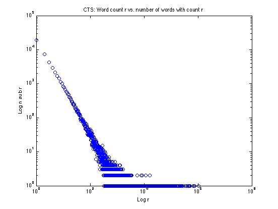
We can see that the low-frequency end looks rather like a straight line on this log-log plot -- why not just fit a line to the straight-looking part and extend it? That's one good solution, and we'll explore things like that in the homework assignment.
But there's an even better idea for how to deal with the quantization of the higher-frequency end of the data, due originally to Bill Gale.
[W]e define a new variable Zr as follows: for any sample frequency r, let r' be the nearest lower sample frequency and r'' the nearest higher sample frequency such that such that nr' and nr'' are both positive rather than zero. Then
Zr = 2nr/(r''-r')
For low r, r' and r'' will be immediately adjacent to r, so that r''-r' will be 2 and Zr will be the same as nr; for high r, Zr will be a fraction, sometimes a small fraction, of nr.
If we calculate these Zr values and plot them as above, it looks like this:
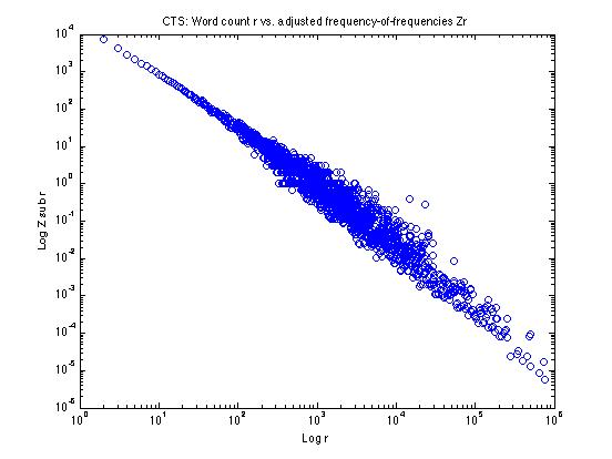
It's still a little fuzzy in parts of the log(r) range -- so we still might want to do some additional smoothing -- but we've pretty well straightened out the effects of the quantization of nr for high r.
To see how and why this works, let's take a look at a few specific values towards the high-r end:
r nr Zr 164,089 1 .0003644 166,066 1 .0001494 177,474 1 .0001078 184,627 1 .0002430 185,703 1 .0004846 188,671 1 .0002435 193,916 1 .0001195 205,408 1 .0000841 217,709 1 .0000829 229,546 1 .0000975 In order to calculate Zr for r=166,066, we do
2*1/(177,474-164,089) = 2/13385 = .0001494
This in effect takes our nr of 1 and smears it out evenly over the whole range from r=164,089 to r=177,474.
Now (perhaps after some additional smoothing) we can calculate r* using Zr instead of nr.
Note that this makes few assumptions about the underlying frequency distribution -- as a result, it will always be more or less applicable, but it might work less well than an approach that makes stronger assumptions -- if the stronger assumptions are true!