Variance, covariance, correlation

 

This continues our exploration of the semantics of the inner product.

As you doubtless know, the variance of a set of numbers is defined as the "mean squared difference from the mean". The inner product of a vector with itself gives us the sum-of-squares part of this, so we can calculate the variance in Matlab like this:

>> X=randn(1000,1);
>> sumsq=(X-mean(X))'*(X-mean(X))    % <- inner product
sumsq =
sumsq =
    1.0293e+03
>> sumsq/1000
ans =
    1.0293

The Matlab function randn() gives us random numbers from a normal distribution with mean 0 and standard deviation of 1. Any particular (random) sample will obviously deviate randomly from this, as in the case where our estimate of the standard deviation is

>> sqrt(sumsq/1000)
ans =
    1.0145

You may know that we're supposed to divide by one less than N to estimate a sample standard deviation. A clue about why this is true is suggested by the case where the sample size N is 1 -- here we really don't want our estimate of the sample variance to be defined at all, whereas if we divide by N, the estimated variance would be zero.

In general, dividing by N introduces a systematic bias into our estimates. Here's a simple way to demonstrate this empirically:

Values=zeros(100,2);
for N=3:100
    M=1000;
    V1=zeros(M,1); V2=zeros(M,1);
    for n=1:M
       X=randn(N,1);
       sumsq=(X-mean(X))'*(X-mean(X));
       V1(n)=(1/N)*sumsq;
       V2(n)=(1/(N-1))*sumsq;
    end
    Values(N,1)=mean(V1);
    Values(N,2)=mean(V2);
end

plot(Values(3:100,1),'bo-')
hold on
plot(Values(3:100,2),'r^-')
hold off

The line with the red triangles, where we've divided the sum of squares by N-1, bobs around above and below 1.0, as it should. The line with the blue circles, where we've divided the sum of squares by N, shows a large bias starting with N=3, getting progressively less biased as N increases:

By the time we get to N=100, it doesn't make much difference any more whether we divide by N or N-1.

In many applications, the concept of covariance comes up. As the name "co+variance" implies, it's like the variance, but applied to a comparison of two vectors: in place of the sum of squares, we have a sum of cross-products:

>> X=randn(100,1); Y=randn(100,1);
>> (1/99)*(X-mean(X))'*(Y-mean(Y))
ans =
      0.0261

(For essentially the same reasons as in the case of the variance, we should divide by N-1 to get an unbiased estimator of the sample covariance.)

Earlier, we looked at the correlation as the inner product of mean-corrected, length-normalized vectors X and Y. An alternative way to look at it is as the covariance of X and Y, divided by the square root of the product of the variance of X and the variance of Y.

Let's set up an example:

% random X and Y vectors:
X=randn(100,1); Y=randn(100,1);
% mean-corrected versions:
xx=X-mean(X); yy=Y-mean(Y);
% covariance and variances:
covXY = (1/99)*xx'*yy
covXY =
         -0.088553915703379
varX = (1/99)*xx'*xx
varX =
          0.848239048469918
varY = (1/99)*yy'*yy
varY =
          1.058702521962021

Now we can compare three ways of getting the correlation r:

covXY/sqrt(varX*varY)
ans =
          -0.093446204270995
%
(xx/sqrt(xx'*xx))'*(yy/sqrt(yy'*yy))
ans =
          -0.093446204270995
%
corr(X,Y)
ans =
          -0.093446204270995

Matlab cov() gives us a matrix of all the variances and covariances:

cov(X,Y)
ans =
         0.848239048469918 -0.088553915703379
        -0.088553915703379 1.058702521962021

But who cares? What is "covariance" good for? For that matter, what is "variance" good for?

We won't attempt a comprehensive answer right away. Instead, let's take a look at how we might use these concepts in a hypothetical case.

We start with 200 random 2-element vectors:

D1 = randn([200 2]);

Matlab randn() selects these a two-dimensional "gaussian" or "normal" distribution, a two-dimensional "bell curve" with a mean of [0 0] and a standard deviation (the square root of the variance) of 1. So what we get is a sort of shotgun-blast of data points:

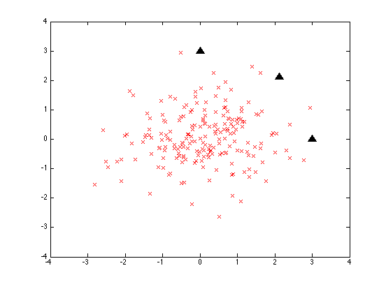
The three black triangles are three points all 3 units away from the origin:

test1 = [0 3; 3*cos(pi/4) 3*sin(pi/4); 3 0];

If we measure their euclidean distance from the origin, all three will be at 3.0 units. If we measure their distance from the mean vector of the random sample, it'll be close to that but not exactly:

>> mean(D1)
ans =
       0.0919 0.0613
>> stest1 = test1 - [mean(D1); mean(D1); mean(D1)]
stest1 =
        2.9081 -0.0613
        2.0294 2.0600
        -0.0919 2.9387

Given those values, the three test points will all be about 2.9 units from the mean of the sample distribution. Given a different random sample, they might have been around 3.1 units away, or some other value -- but their distances will all be close to one another and to 3.0.

Now let's scale the y-axis by a factor of 10 -- as if we were measuring that dimension in millimeters instead of centimeters:

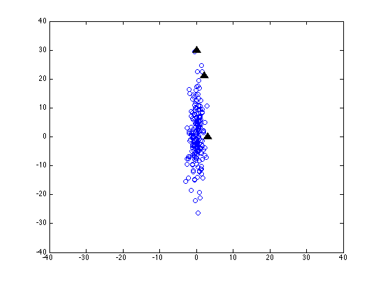
It's all the same data -- and the same test points -- but the values in the second column have all been multiplied by 10.

Now the coordinates of the three test points look like this:

3.0000 0
2.1213 21.2132
0         30.0000

and subtracting the mean vector of the sample (on one random run) we get:

 2.9081   -0.0613
 2.0294    21.1519
-0.0919    29.9387

which gives us euclidean distances of about 2.9, 21.2 and 29.9.

This isn't good -- our axis scaling not only fails to preserve absolute distances, it doesn't even preserve relative distances.

If we were going to use euclidean distance as some kind of similarity measure, this would be a very bad thing. Just changing our units of measurement would screw everything up -- or maybe it was screwed up to start with, since who knows what the "right" units of measurement should be?

One obvious solution to this problem would be to allow the data itself to choose our scale of measurement. And one good way to do that is estimate the standard deviation (the square root of the variance), and then denominate values in terms of distance from the sample mean in standard-deviation units (sometimes known as "z-scores").

But how should be calculate the standard deviation of this two-dimensional data? One obvious thing to try is to do the re-scaling separately in each column.

test2a = test1; test2a(:,2) = test2a(:,2)*10;
sd21 = sqrt(var(D2(:,1))); sd22 = sqrt(var(D2(:,2)));
test2a(:,1) = (test2a(:,1)-mean(D2(:,1)))/sd21;
test2a(:,2) = (test2a(:,2)-mean(D2(:,2)))/sd22;

This looks a good deal better -- the coordinates of our three test points (on one random run) are now:

3.2429 0.0331
2.2897 2.1690
-0.0117 3.0536

and their euclidean distances from the sample's mean vector are 3.2, 3.1 and 3.0 -- which is fine, given the amount of noise introduced by the sampling process.

But what if the coordinate system of our data is not just scaled one axis at a time, but is also rotated? (This will happen whenever we're working with dimensions that are correlated, like height and weight.) Here's our random sample (and our three test points) after we've not only scaled the y axis by a factor of ten, but also rotated things 45 degrees clockwise:

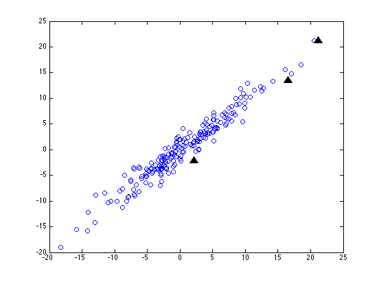
Now before we do any normalization, our three test points are still going to be about 3, 21 and 30 units from the origin (since a rigid rotation doesn't change distances). But this time, even after we re-scale each column in terms of standard-deviations from the mean, the three distances come out as about 0.4, 3.1 and 4.3.

This is a slight improvement -- but I think that you can see that no scaling of the horizontal and vertical axes alone is going to be able to make all the point on our original circle come out with the same distance from the origin. We have to be able to do some squashing or stretching along different directions, which depend on the how the data is arranged.

If all that's happened to our data is squashing, stretching and rotation (also additive shifts, but never mind that for now), then we'll get exactly the right answer if we re-scale things based on the covariance matrix, which represents how the data is distributed not only within but also among the various dimensions of description.

This generalization of the z-transformation was introduced by Prasanta Chandra Mahalanobis in 1936, and is generally called "Mahalanobis distance."

The core of it is a sort of inner product scaled by the inverse of the covarance matrix. If t is the (column) test vector, and m is the mean vector of the sample we're comparing to, and ICM is the inverse of the sample's covariance matrix, then the mahalanobis distance between the test vector and the mean vector will be (in Matlab-ese):

sqrt((t-m)'*ICM*(t-m))

Note that without the ICM term, this would just be the square root of the sum of squared differences, i.e. the euclidean distance.

And if the ICM matrix has the inverse of the variances on the diagonal, and is zero elsewhere, then this becomes just the "normalized euclidean distance" where each dimension is separately scaled by the standard deviation of the sample values on that dimension.

I suggest that you work through in detail what the results of the (t-m)'*ICM*(t-m) product are, in a simple (e.g. 2-dimensional) case. But first, let's show that it's worth the trouble.

In the artificial case we've been investigating, the mahalanobis distances of our three test points come out like this (on one random run):

% Make the random data, scale it, and rotate it:
D1 = randn([200 2]);
s45 = sin(pi/4);
rot45 = [cos(pi/4) -sin(pi/4); sin(pi/4) cos(pi/4)];
D2 = D1; D2(:,2) = D2(:,2)*10;
D3 = D2*rot45;

% Inverse covariance matrix of the scaled, rotated test data:
IC = inv(cov(D3));

% make, scale, rotate 3 test points
test1 = [3 0; 3*s45 3*s45; 0 3];
test2 = test1; test2(:,2) = test2(:,2)*10;
test3 = test2*rot45;

% Calculate the 3 mahalanobis distances:

md1=sqrt(test3(1,:)*IC*test3(1,:)');
md2 = sqrt(test3(2,:)*IC*test3(2,:)');
md3 = sqrt(test3(3,:)*IC*test3(3,:)')

[md1 md2 md3]
ans =
      2.9535 2.9009 2.9820

Not perfect, but a lot better than what we had before.

So go figure out why it works! Or at least, persuade yourself that it does work, and learn how to do it....

On to probabilities

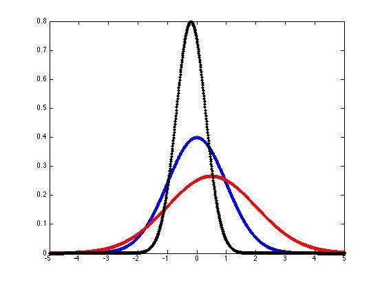
You're probably familiar with the "normal" or "gaussian" probability density function, characterized by a mean μ and a standard deviation σ. The equation looks like this:

And you can plot some sample gaussian pdf's like this:

x = -5:(1/100):5;

mu = 0;
sigma = 1;
k = 1/(sigma*sqrt(2*pi));
y = k*exp(-((x-mu).^2)/(2*sigma^2));
hold off
plot(x,y,'b.-')
hold on

mu = 0.5; sigma = 1.5;

k = 1/(sigma*sqrt(2*pi));
y = k*exp(-((x-mu).^2)/(2*sigma^2));
plot(x,y,'r.-')

mu = -.2; sigma = 0.5;
k = 1/(sigma*sqrt(2*pi));
y = k*exp(-((x-mu).^2)/(2*sigma^2));
plot(x,y,'k.-')

We can generalize these "bell curves" to the case of "multivariate gaussian probability density functions" if we interpret μ as a mean vector rather than a single mean value, replace the standard deviation σ with the covariation matrix Σ, and modify the equation slightly:

Notice the mahalanobis distance lurking inside the exponential...