Tutorial: Pearson's Chi-square Test for Independence

Ling 300, Fall 2008

What is the Chi-square test for?

The Chi-square test is intended to test how likely it is that an observed distribution is due to chance. It is also called a "goodness of fit" statistic, because it measures how well the observed distribution of data fits with the distribution that is expected if the variables are independent.

A Chi-square test is designed to analyze categorical data. That means that the data has been counted and divided into categories. It will not work with parametric or continuous data (such as height in inches). For example, if you want to test whether attending class influences how students perform on an exam, using test scores (from 0-100) as data would not be appropriate for a Chi-square test. However, arranging students into the categories "Pass" and "Fail" would. Additionally, the data in a Chi-square grid should not be in the form of percentages, or anything other than frequency (count) data. Thus, by dividing a class of 54 into groups according to whether they attended class and whether they passed the exam, you might construct a data set like this:

	Pass	Fail
Attended	25	6
Skipped	8	15

IMPORTANT: Be very careful when constructing your categories! A Chi-square test can tell you information based on how you divide up the data. However, it cannot tell you whether the categories you constructed are meaningful. For example, if you are working with data on groups of people, you can divide them into age groups (18-25, 26-40, 41-60...) or income level, but the Chi-square test will treat the divisions between those categories exactly the same as the divisions between male and female, or alive and dead! It's up to you to assess whether your categories make sense, and whether the difference (for example) between age 25 and age 26 is enough to make the categories 18-25 and 26-40 meaningful. This does not mean that categories based on age are a bad idea, but only that you need to be aware of the control you have over organizing data of that sort.

Another way to describe the Chi-square test is that it tests the null hypothesis that the variables are independent. The test compares the observed data to a model that distributes the data according to the expectation that the variables are independent. Wherever the observed data doesn't fit the model, the likelihood that the variables are dependent becomes stronger, thus proving the null hypothesis incorrect!

The following table would represent a possible input to the Chi-square test, using 2 variables to divide the data: gender and party affiliation. 2x2 grids like this one are often the basic example for the Chi-square test, but in actuality any size grid would work as well: 3x3, 4x2, etc.

	Democrat	Republican
Male	20	30
Female	30	20

This shows the basic 2x2 grid. However, this is actually incomplete, in a sense; generally, the data table should include "marginal" information giving the total counts for each column and row, as well as for the whole data set:

	Democrat	Republican	Total
Male	20	30	50
Female	30	20	50
Total	50	50	100

We now have a complete data set on the distribution of 100 individuals into categories of gender (Male/Female) and party affiliation (Democrat/Republican). A Chi-square test would allow you to test how likely it is that gender and party affiliation are completely independent; or in other words, how likely it is that the distribution of males and females in each party is due to chance.

So, as implied, the null hypothesis in this case would be that gender and party affiliation are independent of one another. To test this hypothesis, we need to construct a model which estimates how the data should be distributed if our hypothesis of independence is correct. This is where the totals we put in the margins will become handy: later on, I'll show how you can calculate your estimated data using the marginals. Meanwhile, however, I've constructed an example which will allow very easy calculations. Assuming that there's a 50/50 chance of males or females being in either party, we get the very simple distribution shown below.

	Democrat	Republican	Total
Male	25	25	50
Female	25	25	50
Total	50	50	100

This is the information we would need to calculate the likelihood that gender and party affiliation are independent. I will discuss the next steps in calculating a Chi square value later, but for now I'll focus on the background information.

Note: you can assume a different null hypothesis for a Chi-square test. Using the scenario suggested above, you could test the hypothesis that women are twice as likely to register as Democrats than men, and a Chi-square test would tell you how likely it is that the observed data reflects that relationship between your variables. In this case, you would simply run the test using a model of expected data built under the assumption that this hypothesis is true, and the formula will (as before) test how well that distribution fits the observed data. I will not discuss this in more detail, but it is important to know that the null hypothesis is not some abstract "fact" about the test, but rather a choice you make when calculating your model.

What is the Chi-square test NOT for?

This is also an important question to tackle, of course. Using a statistical test without having a good idea of what it can and cannot do means that you may misuse the test, but also that you won't have a clear grasp of what your results really mean. Even if you don't understand the detailed mathematics underlying the test, it is not difficult to have a good comprehension of where it is or isn't appropriate to use. I mentioned some of this above, when contrasting types of data and so on. This section will consider other things that the Chi-square test is not meant to do.

First of all, the Chi-square test is only meant to test the probability of independence of a distribution of data. It will NOT tell you any details about the relationship between them. If you want to calculate how much more likely it is that a woman will be a Democrat than a man, the Chi-square test is not going to be very helpful. However, once you have determined the probability that the two variables are related (using the Chi-square test), you can use other methods to explore their interaction in more detail. For a fairly simple way of discussing the relationship between variables, I recommend the odds ratio.

Some further considerations are necessary when selecting or organizing your data to run a Chi-square test. The variables you consider must be mutually exclusive; participation in one category should not entail or allow participation in another. In other words, the data from all of your cells should add up to the total count, and no item should be counted twice.

You should also never exclude some part of your data set. If your study examined males and females registered as Republican, Democrat, and Independent, then excluding one category from the grid might conceal critical data about the distribution of your data.

It is also important that you have enough data to perform a viable Chi-square test. If the estimated data in any given cell is below 5, then there is not enough data to perform a Chi-square test. In a case like this, you should research some other techniques for smaller data sets: for example, there is a correction for the Chi-square test to use with small data sets, called the Yates correction. There are also tests written specifically for smaller data sets, like the Fisher Exact Test.

Degrees of Freedom

A broader description of this topic can be found here.

The degrees of freedom (often abbreviated as df or d) tell you how many numbers in your grid are actually independent. For a Chi-square grid, the degrees of freedom can be said to be the number of cells you need to fill in before, given the totals in the margins, you can fill in the rest of the grid using a formula. You can see the idea intended; if you have a given set of totals for each column and row, then you don't have unlimited freedom when filling in the cells. You can only fill in a certain amount of cells with "random" numbers before the rest just becomes dependent on making sure the cells add up to the totals. Thus, the number of cells that can be filled in independently tell us something about the actual amount of variation permitted by the data set.

The degrees of freedom for a Chi-square grid are equal to the number of rows minus one times the number of columns minus one: that is, (R-1)*(C-1). In our simple 2x2 grid, the degrees of independence are therefore (2-1)*(2-1), or 1! Note that once you have put a number into one cell of a 2x2 grid, the totals determine the rest for you.

Degrees of freedom are important in a Chi-square test because they factor into your calculations of the probability of independence. Once you calculate a Chi-square value, you use this number and the degrees of freedom to decide the probability, or p-value, of independence. This is the crucial result of a Chi-square test, which means that knowing the degrees of freedom is crucial!

Building a Model of Expected Data

Earlier, I showed a simple example of observed vs. expected data, using an artificial data set on the party affiliations of males and females. I show them again below.

Observed

	Democrat	Republican	Total
Male	20	30	50
Female	30	20	50
Total	50	50	100

Expected (assuming independence)

	Democrat	Republican	Total
Male	25	25	50
Female	25	25	50
Total	50	50	100

We will focus on models based on the null hypothesis that the distribution of data is due to chance -- that is, our models will reflect the expected distribution of data when that hypothesis is assumed to be true. But as I mentioned before, the ease of dividing up this data is due to the simplicity of the distribution I chose. How do we calculate the expected distribution of a more complicated data set?

	Pass	Fail	Total
Attended	25	6	31
Skipped	8	15	23
Total	33	21	54

Here is the grid for an earlier example I discussed, showing how students who attended or skipped class performed on an exam. The numbers for this example are not so clean! Fortunately, we have a formula to guide us.

The estimated value for each cell is the total for its row multiplied by the total for its column, then divided by the total for the table: that is, (RowTotal*ColTotal)/GridTotal. Thus, in our table above, the expected count in cell (1,1) is (33*31)/54, or 18.94. Don't be afraid of decimals for your expected counts; they're meant to be estimates!

I'll show a different method for notating observed versus expected counts below: the expected frequency appears in parentheses below the observed frequency. This allows you to show all your data in one clean table.

	Pass	Fail	Total
Attended	25 (18.94)	6 (12.05)	31
Skipped	8 (14.05)	15 (8.94)	23
Total	33	21	54

We have now calculated the distribution of our totals based on the assumption that attending class will have absolutely no effect on your test performance. Let's all hope we can prove this null hypothesis wrong.

The Chi-square Formula

It's finally time to put our data to the test. You can find many programs that will calculate a Chi-square value for you, and later I will show you how to do it in Excel. For now, however, let's start by trying to understand the formula itself.

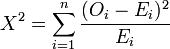
What does this mean?? Actually, it's a fairly simple relationship. The variables in this formula are not simply symbols, but actual concepts that we've been discussing all along. O stands for the Observed frequency. E stands for the Expected frequency. You subtract the expected count from the observed count to find the difference between the two (also called the "residual"). You calculate the square of that number to get rid of positive and negative values (because the squares of 5 and -5 are, of course, both 25). Then, you divide the result by the expected frequency to normalize bigger and smaller counts (because we don't want a formula that will give us a bigger Chi-square value just because you're working with a bigger set of data). The huge sigma sitting in front of all that is asking for the sum of every i for which you calculate this relationship - in other words, you calculate this for each cell in the table, then add it all together. And that's it!

Using this formula, we find that the Chi-square value for our gender/party example is ((20-25)^2/25) + ((30-25)^2/25) + ((30-25)^2/25) + ((20-25)^2/25), or (25/25) + (25/25) + (25/25) + (25/25), or 1 + 1 + 1 + 1, which comes out to 4.

Okay, but what does THAT mean?? In a sense, not much yet. The Chi-square value serves as input for the more interesting piece of information: the p-value. Calculating a p-value is less intuitive than a Chi-square value, so I will not discuss the actual formula here, but simply tools to use in calculating this data. We will need the following to get a p-value for our data:

(1) The Chi-square value.
(2) The degrees of freedom.

Once you have this information, there are a couple of methods you can use to get your p-value. For example, charts like this one or even Javascript programs like the one on this site will take the Chi-square value and degrees of freedom as input, and simply return a p-value. In the chart, you choose your degrees of freedom (df) value on the left, follow along its row to the closest number to your Chi-square value, and then check the corresponding number in the top row to see the approximate probability ("Significance Level") for that value. The Javascript program is more direct, as you simply input your numbers and click "calculate." Later, I will also show you how to make Excel do the work for you.

So, for our example, we take a Chi-square value of 4 and a df of 1, which gives us a p-value of 0.0455. This is interpreted as a 4.6% likelihood that the null hypothesis is correct. To put it best, if the distribution of this data is due entirely to chance, then you have a 4.6% chance of finding a discrepancy between the observed and expected distributions that is at least this extreme.

By convention, the "cutoff" point for a p-value is 0.05; anything below that can be considered a very low probability, while anything above it is considered a reasonable probability. However, that does not mean that we should take our 0.046 value and say, "Eureka! They're dependent!" Actually, 0.046 is so close to 0.05 that there's really not much we can say from this example; it is teetering right on the brink of chance. This is a very good thing to realize, because from this we discover that although the distribution seems to have fairly clear tendencies in certain directions when you just look at it, the data shows that it's not so unlikely that this would show up just by chance.

So, let's try our other data set, and see if attending class really does affect your exam performance.

	Pass	Fail	Total
Attended	25 (18.94)	6 (12.05)	31
Skipped	8 (14.05)	15 (8.94)	23
Total	33	21	54

I'm going to skip the specific formula this time, and use the javascript program on this site to do the calculation for me. It returns a value of 11.686. We still only have 1 degree of freedom, so our p-value is calculated as 0.0006. In other words, if this distribution was due to chance, we would see exactly this distribution only 0.06% of the time! A value of 0.0006 is a much lower probability than a value of 0.05. We can thus safely say that the null hypothesis is incorrect; attending class and passing the exam are definitely dependent on one another. (Of course, if you are testing a null hypothesis that you are expecting to be correct, then you would want a very high p-value. The reason we want a low one in this case is because we are trying to disprove the hypothesis that the variables are independent.)

This is all you need to know to calculate and understand Pearson's Chi-square test for independence. It's a widely popular test because once you know the formula, it can all be done on a pocket calculator, and then compared to simple charts to give you a probability value. You can also use this spreadsheet to play around with all the steps of the test (spreadsheet created by Bill Labov, with some small additions by Joel Wallenberg). The Chi-square test will prove to be a handy tool for analyzing all kinds of relationships; once you know the basics for a 2x2 grid, expanding to a larger set of values is easy. Good luck!